Mechanism of Differential Privacy

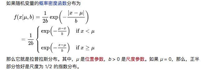
Laplace Distribution

The following details are from Wikipedia. And the python version is here

PDF

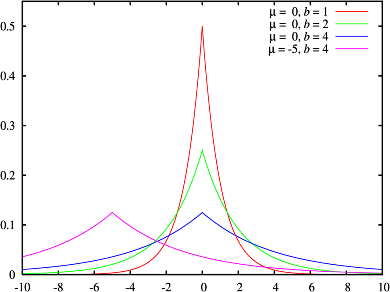
1. 概率密度函数反映了概率在$ x$点处的密集程度。
2. x轴表示每一种取值，而y轴表示概率。
3. the variance of this distribution is $\sigma^2=2b^2$, while its scale is $b$.

CDF

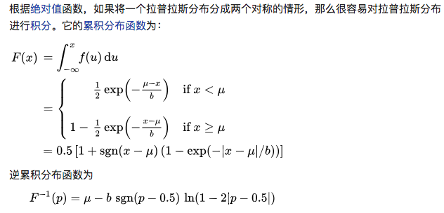
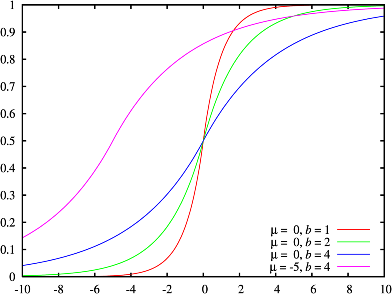
1. CDF表示连续累积概率，即$F(0)=P(x\le{0})$，即所有非正值的概率和。
2. PDF 表示某一点取值的概率$f(0)=P(x=0)=0.5$

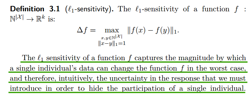
Sensitivity

L1-sensitivity

Remarks:

1. $N^{|X|}$ 表示数据库的大小是$|X|$, 即有$X$条记录；而$\mathbb{R}$表示real number，$\mathbb{R}^{k}$则表示$k$维空间，即数据是$k$维的，$k$维向量。

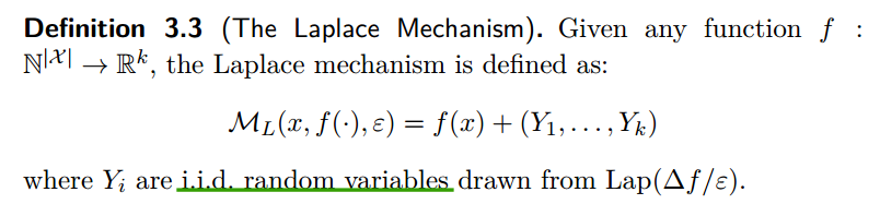
Laplace Mechanism

TO DO QUESTION??

1. WHY LAPLACE DISTRIBUTION????

2. WHY SENSITIVITY IN THE SCALE????

Definition

the Laplace mechanism will simply compute $f$, and perturb each coordinate with noise drawn from the Laplace distribution.

About the proof, the key is that :

1. neighbourhood database:

   $x\in{N^{|X|}}$ and $y\in{N^{|X|}}$, such that $||x-y||_1=\le1$.

2. noise result:

   $\frac{P(f(x)=z)}{P(f(y)=z)}\le{e^{\epsilon}}$

Remarks:

1. Let $\hat{f(x)}$ be the output of Laplace mechanism with zero mean given an input $x$. Then, for ant $x$, $\mathbb{E}[\hat{f(x)}]=f(x)$, where $f(x)$ is true query result without any perturbation.

   $\mathbb{E}[\hat{f(x)}]=\int{P(x)}\hat{f(x)}dx=\int{P(x)(f(x)+n(x))}dx=f(x)\int{P(x)}dx+\int{P(x)n(x)}dx$

   Obviously, $\int{P(x)}dx=1$, since the distribution of $n$ has zero mean so it is symmetric. For any $Pr(x)$, there are always two variables $n_1$ and $n_2$ such that $n_2=-n_1$, resulting in $P(n_1)n_1+P(n_2)n_2=0$. So $\int{P(x)n(x)}dx=0$.

   SO $\mathbb{E}[\hat{f(x)}]=f(x)$

2. The error introduced by $Lap(0,\frac 1 \epsilon) \ is\ \frac 1 \epsilon​$

   Assume $X$ is true answer and $Y=X+n$ is the noise output. $Error^2=E((Y-X)^2)=E(n^2)=E((n-E(n))^2)=E((n-0)^2)=Var(n)$

   so the variance of noise distribution is the error, which is $\sqrt 2 b=\sqrt 2 \frac{1}{\epsilon}$

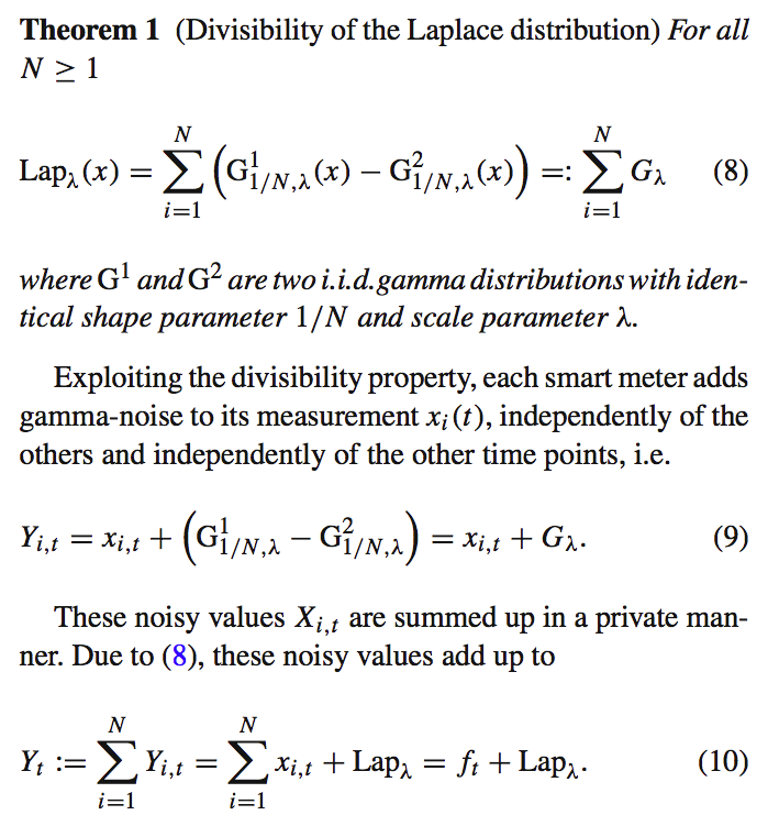
Properties

Divisibility of Laplace Distribution

Python Implement

def noise():
    loc = 0
    scale = 1
    noise = np.random.laplace(loc,scale,1) #返回一个list
    return noise[0]

Examples

We sometimes refer to the problem of responding to large numbers of (possibly arbitrary) queries as the query release problem.

1. Counting Queries

   Since the sensitivity of a counting query is 1 (the addition or deletion of a single individual can change a count by at most 1), so $(\epsilon,0)$-differential privacy can be achieved for counting queries by the addition of noise scaled to $\frac{1}{\epsilon}$, that is, by adding noise drawn from Lap($\frac{1}{\epsilon}$). The expected distortion, or error, is $\frac{1}{\epsilon}$, independent of the size of the database.

   A fixed but arbitrary list of m counting queries can be viewed as a vector-valued query. Absent any further information about the set of queries a worst-case bound on the sensitivity of this vector-valued query is m, as a single individual might change every count. In this case $(\epsilon,0)$-differential privacy can be achieved by adding noise scaled to $\frac{m}{\epsilon}$ to the true answer to each query.

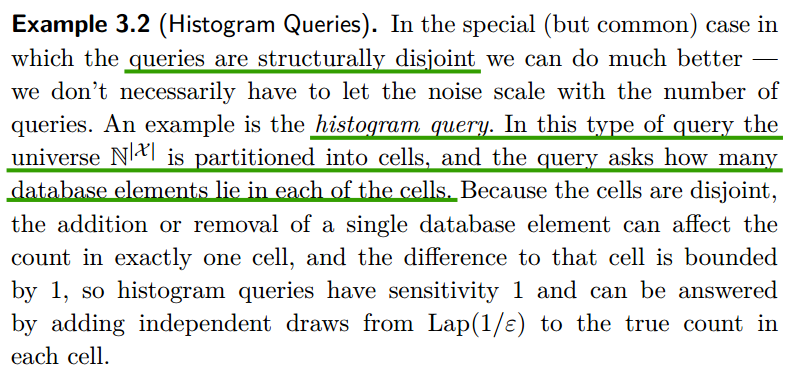
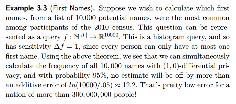
2. Histogram Queries

   

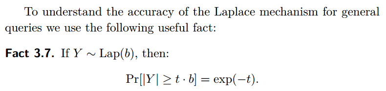
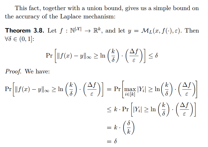
Utility

Remarks:

1. Theorem3.8中，Pr[]里面，左边表示Laplace mechanism产生的error，右边中的两项，$t=In(\frac{k}{\delta})$，$k$是query result的维度，$b=\frac{\Delta{f}}{\epsilon}$。
2. 

Exponential mechanism

The exponential mechanism was designed for situations in which we wish to choose the “best” response but adding noise directly to the computed quantity can completely destroy its value, such as setting a price in an auction, where the goal is to maximize revenue, and adding a small amount of positive noise to the optimal price (in order to protect the privacy of a bid) could dramatically reduce the resulting revenue.

Definition

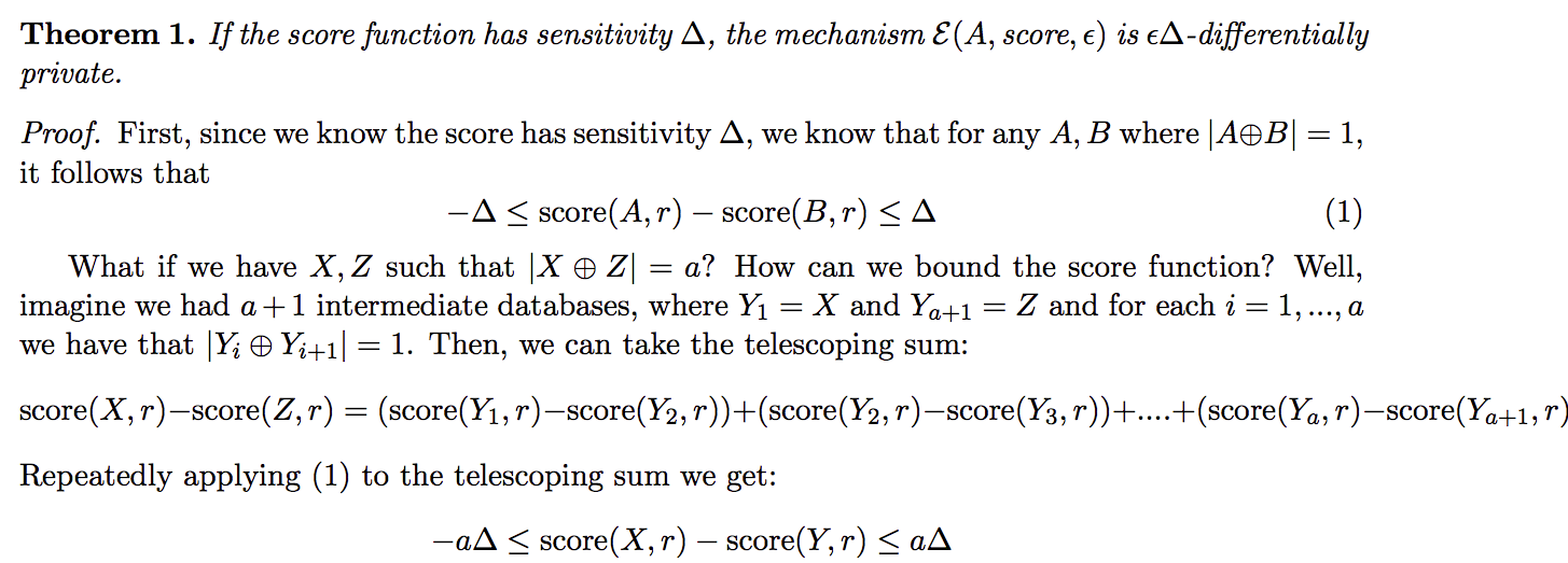
The sensitivity of score function $q$ tells us the maximum change in the scoring function for any pair of datasets $d$ and $d’$ such that $|d\otimes d’|=1$:

$$\Delta q = max_{r,d,d' where |d\otimes d'|=1 }|q(d,r)-q(d',r)|$$

Say we have a discrete candidate output in a range $R$, and assume that the probability distribution of output is $u$, commonly uniform. The general mechanism is to design a query function $q:D^n(input)\times{R(output)}\to{\mathbb{R}}$, which assign a real valued score to any pair $(d,r)$ from $D^n\times{R}$. With a prior distribution of candidate output $u$, we amplify the probability associated with each output by a factor of $e^{\epsilon{q(d,r)}}$:

$$\Delta{q}=max_{r\in{R}}\ max_{x,y:||x-y||_1\le{1}}|q(x,r)-q(y-r)|$$

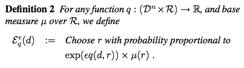
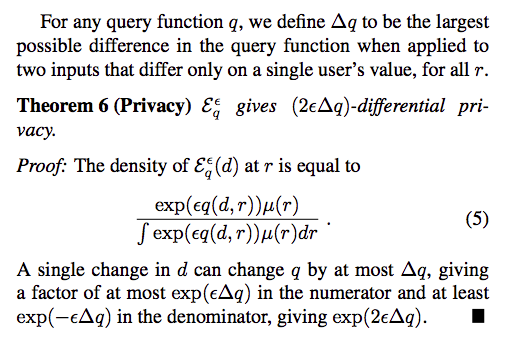
Remarks:

1. by amplifying the probability, the sum of all output probability will not equal 1. So in order to bound the probability, we need a normalization term.

2. from the denifition, if we set the probability factor as $\epsilon$, then it will provide us $2\epsilon \Delta q$, which amptifies with a factor $2\Delta q$. SO if we want $\epsilon$-DP, then the probability factor should be $\frac{\epsilon}{2\Delta q}$

3. the exponential mechanism defines a distribution over the output domain and samples from this distribution.

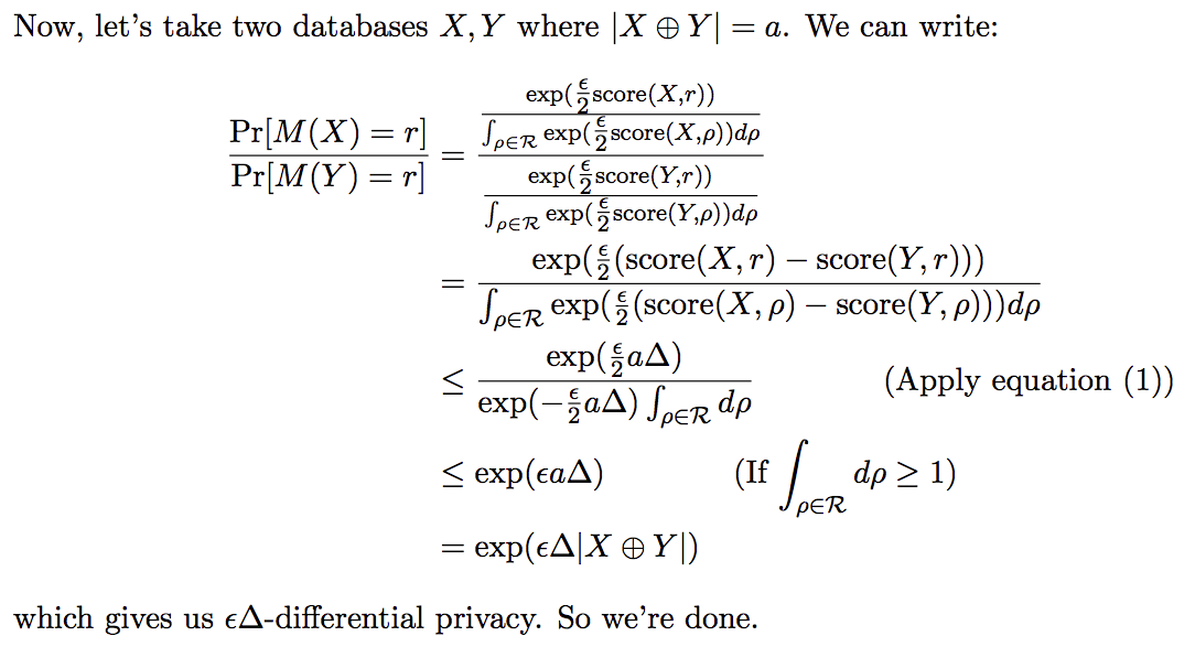
4. now we want to know how a small change in the database can affect the output. Say we have database $d$ and $d’$, where $||d-d’||=1$. And we assume $q(d,r)=q(d’,r)+\Delta{q}$. we want to bound the probability ratio $\frac{P(r|d)}{P(r|d’)}$

   $$\begin{equation} \begin{aligned} \frac{P(r|d)}{P(r|d')}&=\frac{e^{\epsilon{q(d,r)}}}{\int{e^{\epsilon{q(d,r)}}}}\div\frac{e^{\epsilon{q(d',r)}}}{\int{e^{\epsilon{q(d',r)}}}}\\ &=\frac{e^{\epsilon{q(d,r)}}}{e^{\epsilon{q(d',r)}}}\times\frac{\int{e^{\epsilon{q(d',r)}}}}{\int{e^{\epsilon{q(d,r)}}}}\\ for\ the\ left\ one,\ we\ replace\ q(d,r)=q(d',r)+\Delta{q} ,\\ for\ right\ since\ q(d',r)= q(d',r)-q(d,r)+q(d,r) \\ &={\frac{e^{\epsilon{(q(d',r)+\Delta{q})}}}{e^{\epsilon{q(d',r)}}}}\times\frac{\int{e^{\epsilon{(q(d',r)}-\epsilon{(q(d,r)+\epsilon{(q(d,r)}})}}} {\int{e^{\epsilon{q(d,r)}}}}\\ since\ |q(d',r)-q(d,r)|\le \Delta q,\ so\ we\ have \\ &\le e^{\epsilon \Delta q} \times \int{e^{\epsilon \Delta q}}\\ &=e^{\epsilon \Delta q}\times{e^{\epsilon{\Delta{q}}}}\\ &=e^{2\epsilon \Delta q} \end{aligned} \end{equation}$$

Utility

The exponential mechanism can often give strong utility guarantees, because it discounts outcomes exponentially quickly as their quality score falls off.

Let $OPT_{q}(d)=max_{r\in R}q(d,r)$ denote the maximum score of any candidate output $r\in R$ with respect to database $d$.

Fixing a database $d$, let $R_{OPT}=\{r\in R:q(d,r)=OPT_{q}(x)\}$ denote the set of candidates in $R$ which attain maximum utility score $OPT_q(x)$. Then:

Theorem:

$$Pr[q(M_{E(d,q,R)}\le OPT_q(d)-\frac{2\Delta q}{\epsilon}(ln(\frac{|R|}{|R_{OPT}|})+t))]\le e^{-t}$$

Corollary:

$$Pr[q(M_{E(d,q,R)}\le OPT_q(d)-\frac{2\Delta q}{\epsilon}(ln(|R|)+t))]\le e^{-t}$$

Remarks:

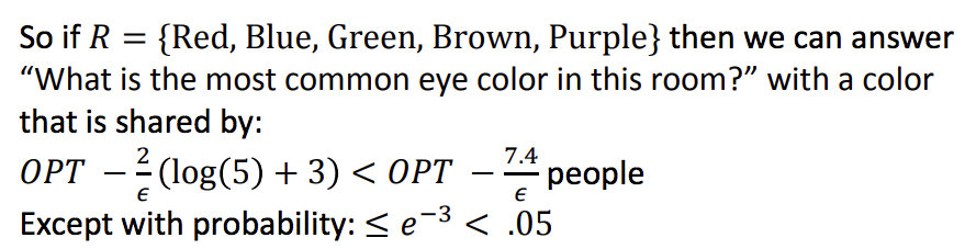
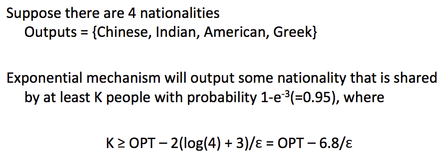
1. We bound the probability that the exponential mechanism returns a “good” output of $R$, where good is measured in terms of $OPT_q(d)$. The result is that it will be highly unlikely that the returned output $r$ has a utility score that is inferior to $OPT_q(x)$ by more than an additive factoc of $O(\frac{\Delta q}{\epsilon}log|R|)$
2. from the utility theorem, we can find that utility of the mechanism only depends on log(|Outputs|), leading to the fact that sampling an output may not be computationally efficient if output space is large.
3. 
4. 

Laplace vs Exponential

Exponential mechanism is an instance of the exponential mechanism.

1. candidate output domain

   Say we have the output domian $r\in R$, and the query function is $f$ which works over the database $d$ and $d’$ such that $|d\otimes{d’}|=1$.

2. utility function

   $$q(d,r)=-|f(d)-r|$$

   To see how this works, notice first that with this scoring function, the exponential mechanism becomes:

   $M(d,q,\epsilon)$=output $r$ with probability proportional to $e^{\epsilon q(d,r)}$

   which provides $2\epsilon \Delta q$-DP.

3. sensitivity

   $$\begin{equation} \begin{aligned} \Delta q &=max|q(d,r)-q(d',r)|\\ &=max||f(d')-r|-|f(d,r)||\\ &\le max|f(d',r)-f(d,r)| \ \ \ \ \ \ \ \ \ \ \ \ \ \ (triangle inequlity)\\ \end{aligned} \end{equation}$$

   So based on above details, for query function with sensitivity 1 and with privacy parameter $\epsilon$, exponential mechanism provides $2\epsilon$-DP, while Laplace mechanism provides $\epsilon$-DP. This is because we’ve used the general analysis of the exponential mechanism, so our result is less “tight”.

   This means that to provide the same privacy level $\epsilon$, laplace mechanism is $\epsilon-$DP while exponential mechanism is $\frac{\epsilon}{2}$-DP, meaning more noise.

Examples

The median mechanism

Recall that the median of a list numbers $d=\{1,2,4,5,6\}$ is 4; so we write $med(d)=4$

1. candidate ooutputs

   every element in $d$ is the possilble output of the median query.

2. utility function

   For the median example, our scoring function will be:

   $q(d,r)=-min|d\otimes d’|$ such that $med(d’)=r$

   What does it mean? The idea is that we take in a database $d$ and a candidate median $r$, and we look for a $d’$ that is as similar as possible to $d$, such that $med(d’)=r$.

   For example, $d=\{1,2,3,4,5\}$ and candidate output $r=4$. What we want to do is to change $d$ to $d’$ so that $med(d’)=4$. To do so, we can remove $1$ and $2$ from the $d$ to get $d’=\{3,4,5\}$. so $q(\{1,2,3,4,5\},4)=-2$. If $r=3$, $q(\{1,2,3,4,5\},4)=0$ becasue $3$ is the true median and we needn’t change anything about database $d$.

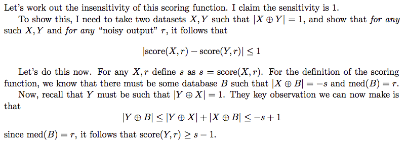
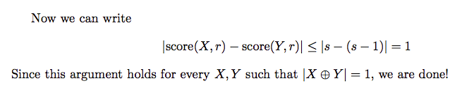
3. sensitivity

   We can get $|q(d,r)-q(d’,r)|\le 1$. It is obvious because the input database is added or removed one element, for the unchanged database, the change you make to make $r$ median is $x$ step. Now we have already help you make a step. So the best situation is you only need to maek (x-1) step for x as median. The utility change is 1. While the worst situation is the addition or removal in the original database don’t help you at all, so you still need $x$ step. So the utility change is 0.

   There is the mathametical proof.

   

   

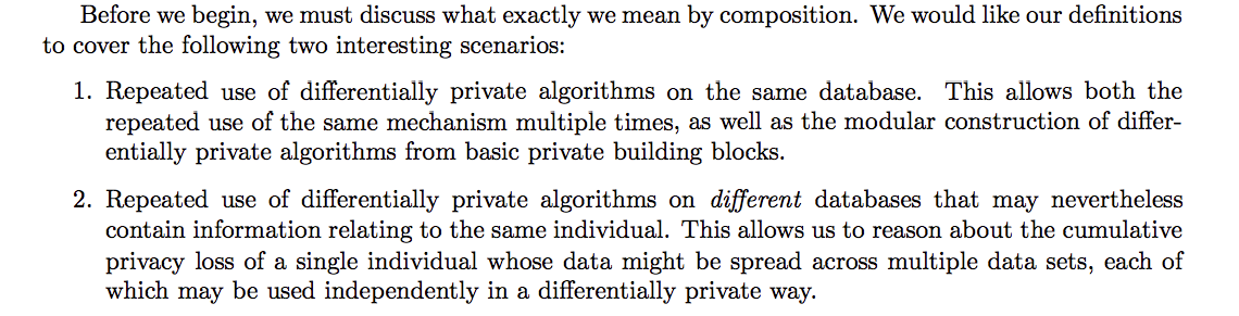
Composition Theorems

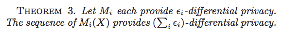
[2009-McSherry] Any approach to privacy must address issues of composition: that several outputs may be taken together, and should still provide privacy guarantees even when subjected to joint analysis

[2014-Dwork] The combination of two differentially private algorithms is differentially private itself. But the parameters $\epsilon$ and $\delta$ will necessarily degrade —- consider repeatedly computing the same statistic using the Laplace mechanism. The average of the answer given by each instance of the mechanism will eventually converge to the true value of the statistic, and so we cannot avoid that the strength of our privacy guarantee will degrade with repeated use.

Sequential composition

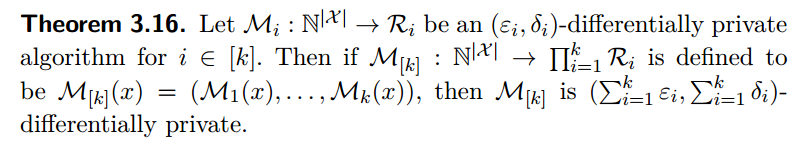
Proof:

$$\begin{equation} \begin{aligned} Pr(M(X)=O)& =\prod_{i=1}^{m}Pr(M_i(X)=O_i) \\ &\le \prod_{i=1}^{m} e^{\epsilon_i}Pr(M_i{(X')=O_i})\\ &=e^{\sum_{i=1}^{m}\epsilon_i}\prod_{i=1}^{m} Pr(M_i(X')=O_i)\\ &=e^{\sum_{i=1}^{m}\epsilon_i} Pr(M_i(X)=O) \end{aligned} \end{equation}$$

x

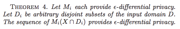
Parallel composition

While general sequences of queries accumulate privacy costs additively, when the queries are applied to disjoint subsets of the data we can improve the bound. Specifically, if the domain of input records is partitioned into disjoint sets, independent of the actual data, and the restrictions of the input data to each part are subjected to differentially-private analysis, the ultimate privacy guarantee depends only on the worst of the guarantees of each analysis, not the sum.

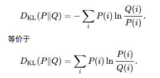
KL-Divergence

又叫相对熵，是衡量分布间距离的一个度量。

定义

设$P(i)​$和$Q(i)​$是$X​$取值的两个概率分布，则$P​$相对$Q​$的KL-Divergence是：

性质

1. 非对称性

   $$D(p||q)\ne{D(q||p)}$$

2. 非负性

   $$D(p||q)\ge0$$

[2011-Aaron]

Reference

[2014-Dwork] The Algorithmic Foundations of Differential Privacy

[2006-Dwork] Calibrating Noise to Sensitivity in Private Data Analysis

[2009-McSherry] Privacy Integrated Queries

[2016-Gunther Eibl] Differential privacy for real smart metering data