Statistic 110

This post is about my learning process of probability and statistics.

Probabilistic Systems Analysis and Applied Probability

last time

[Fundamentals of Probability]

[Discrete Stochastic Processes]

Mathematics for Computer Science

open course

homework with solutions

Probability

This chapter is based on the book “Mathematics for Computer Science”.

Event and Probability

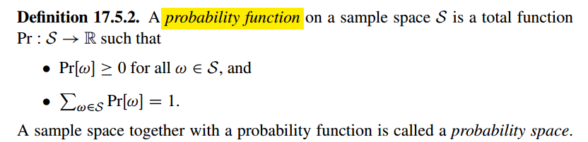
Definition

A countable sample space $S$ is a nonempty countable set. An element $w \in S$ is called an outcome. A subset of $S$ is called an event.

The Four Step Method

In order to understand what event and probability are, we are going to introduce a problem and solve with a four-step method.

Suppose you’re on a game show, and you’re given the choice of three doors. Behind one door is a car, behind the others, goats. You pick a door, say number 1, and the host, who knows what’s behind the doors, opens another door, say number 3, which has a goat. He says to you, “Do you want to pick door number 2?” Is it to your advantage to switch your choice of doors?

In order to answer this question, we want to know whether we can increase the possibility of winning by switching the door. Therefore, our goal becomes probability computation and The-Four-Step-Method is commonly used to perform this task.

Step 1: Find the Sample Space

In this step, our goal is to determine the all the possible outcomes of the experiments. A typical experiment usually involves several steps. For example, in our problem setting, our experiment has the following steps:

1. Put a car in a random door.
2. Pick a door.
3. Open another door with a goat behind it.

Every possible combination of these randomly-determined quantities is called an
outcome. The set of all possible outcomes is called the sample space for the experiment.

Considering the small sample space in this experiment, we are going to use a tree structure to represent the whole space.

Specifically, for the first step: put a car in a random door. Since there are three available door, so we have three possibilities:

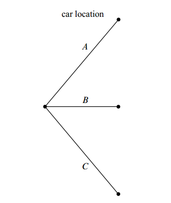
Here, A, B and C are door names.

In the second step, for each car possible location, a user have three possible way to choose a door which he thinks the car is behind:

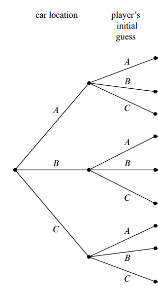
In the final step, we try to reveal a door with a goat behind it. For example, say the car is behind door A and the user choose the door A, then we can reveal either of the doors, i.e., B or C, since goats are both behind these two doors. But if the car is in location A and the user choose the door B, then we can only reveal the door C. The full tree structure is as following:

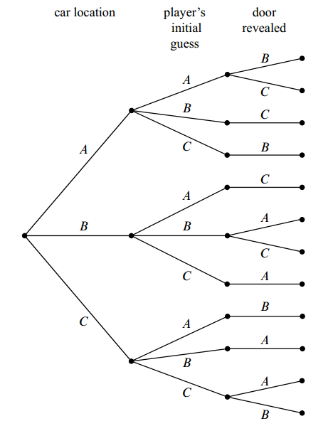
Now let’s relate this picture to the terms we introduced earlier: the leaves of the
tree represent outcomes of the experiment, and the set of all leaves represents the
sample space.

Thus in this experiment, there are 12 outcomes. If we represent each outcome in the format: (door with car, door chosen, door opened with a goat behind), we have the sample space :

Step 3: Define Events of Interest

A set of outcomes is called an event. Each of the preceding phrases characterizes
an event. For example, the event [prize is behind door C] refers to the set:

$$\{(C,A,B),(C,B,A),(C,C,A),(C,C,B)\}$$

and the event [prize is behind the door first picked by the player] is:

$$\{(A,A,B),(A,A,C),(B,B,A),(B,B,C),(C,C,A),(C,C,B)\}$$

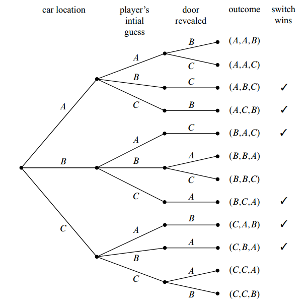
Remember our goal is the probability of wining if the user switches the door, so the door with prize is different from the door opened, i.e., the 1st element is different from the 3rd element of an outcome; and since we are going to switch the door, so the door chosen is differnt the door opened, i.e., the three elements of an outcome should be different. Therefore, this event can be represented by:

$$\{(A,B,C),(A,C,B),(B,A,C),(B,C,A),(C,A,B),(C,B,A)\}$$

We can mark the outcomes in the tree diagram:

Step 3: Determine Outcome Probabilities

The goal of this step is to assign each outcome a probability, indicating the fraction of the time this outcome is expected to occur. And the sum of all the outcome probabilities must equal one, reflecting the fact that there must be an outcome. We are going to break the task of determining outcome probabilities into two stages.

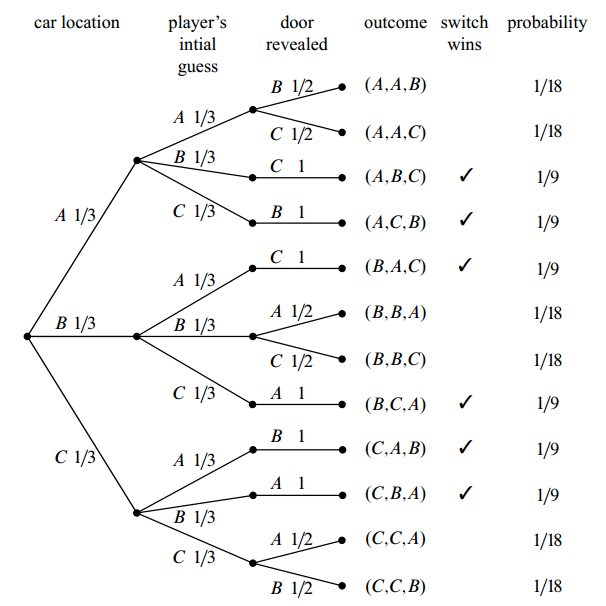
1. Assign Edge Probabilities

   For example, for the car location field, probability of car behind door A is $\frac{1}{3}$, so we assign $\frac{1}{3}$ to that edge. Then for the player’s initial guess, the probability of each choice is also $\frac{1}{3}$. Say the player choose door A, then for door revealed filed, each possibility is $\frac{1}{2}$. But if the player choose the door B, then we can only reveal door C, so the probability is 1.

2. Compute Outcome Probabilities

   For each outcome, we multiply the edge probability and get the probability of this outcome.

   

Step 4: Compute Event Probabilities

Now we have the probability of each outcome, so we can compute an event probability by adding all the outcome probability of that event.

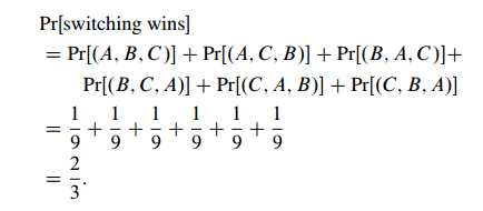
It means that we have the $\frac{2}{3}$ probability to win if we switch the doors.

Independence

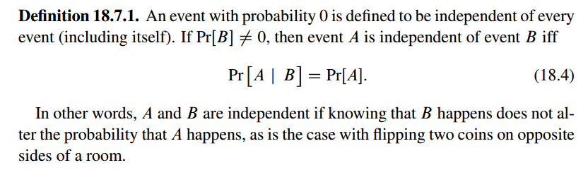
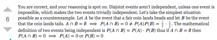
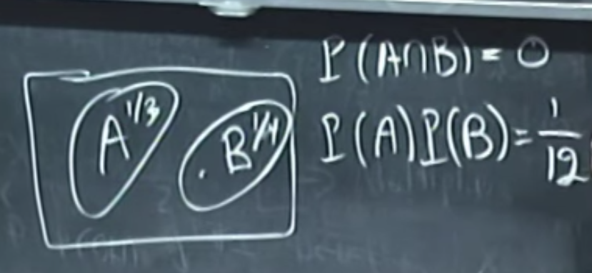
Based on the pic, $P(AB)\ne P(A)P(B)$, so event A and event B are not independent event.

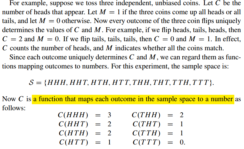
Random Variables

Definition A random variable $R$ is a function, mapping the sample space to a number.

Example

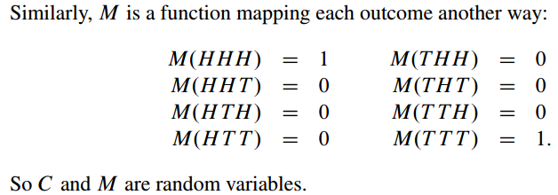
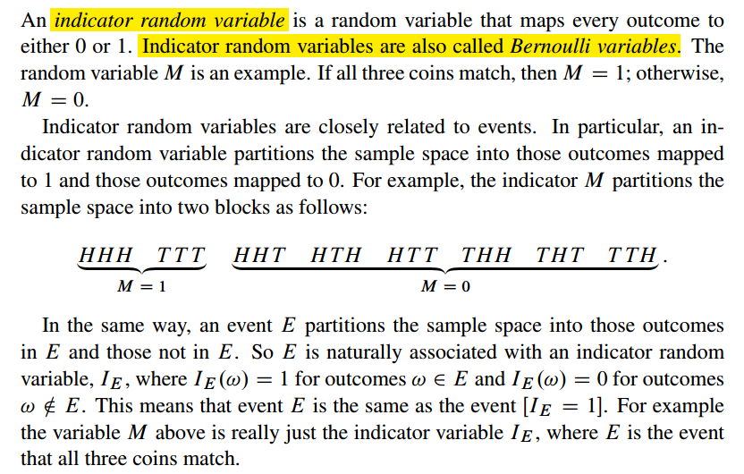
Indicator Random Variables

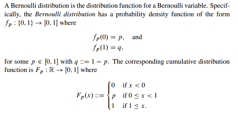
Distribution Functions

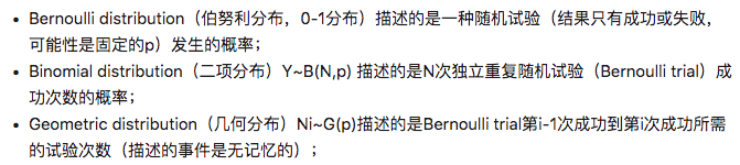
Bernoulli Distributions

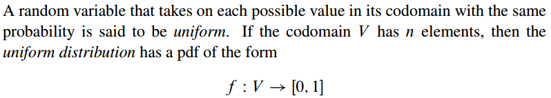
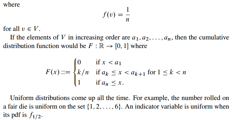
Uniform Distributions

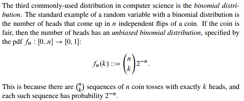
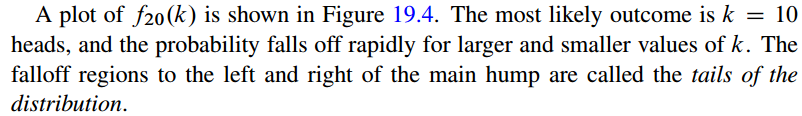
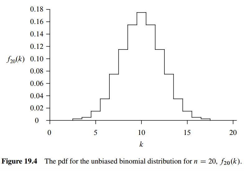
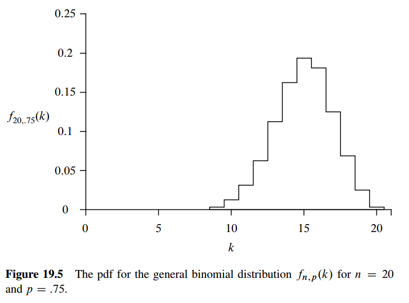
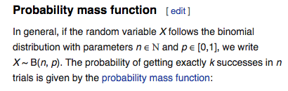
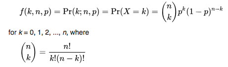
Binomial Distributions

Expectations

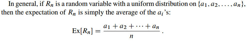
The Expected Value of a Uniform Random Variable

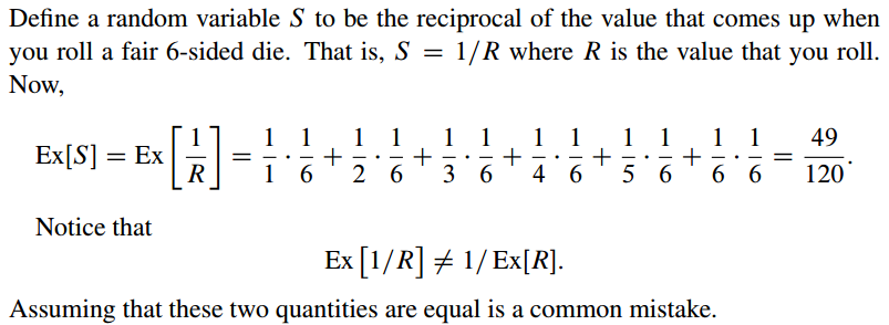
The Expected Value of a Reciprocal Random Variable

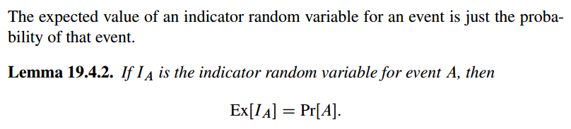
The Expected Value of an Indicator Random Variable

Discrete Random Variables

1. Probability mass function (PMF)

   it is the probability of a discrete random variable; while in continus setting, the probability of a random variable is called PDF.

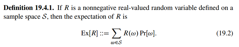
2. Expectation

   $$E(X)=\sum_{x}xp_X(x)$$

   • Average in large number of repetitions the experiment

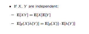
3. Properties of expectations

   

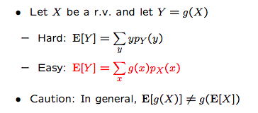
   • Once x is determined, then y is determined; so the probability of y is the probability of x;

   If $\alpha , \beta$ are constants, then:

   $$E(\alpha)=\alpha\\ E(\alpha X)=\alpha E(X)\\ E(\alpha X+\beta)=\alpha E(X)+\beta$$

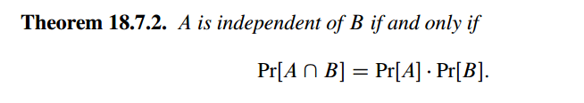
   But if A and B are two independent variables, then

   $$\begin{equation} \begin{aligned} E(AB)&=\sum_A\sum_B(ab)P_{A,B}(a,b)\\ &=\sum_A\sum_B(ab)P_A(a)P_B(b) \\&=E(A)E(B) \end{aligned} \end{equation}$$

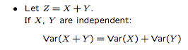
4. Variance

   

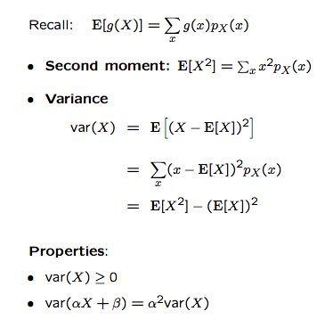
   • since $X$ is random while $E(X)$ is a number, so $X-E(X)$ is a random variable.
   • variance measures the average square distance from the mean.
   • a big variance means the variable are far away from the center while a small one means the variables are tightly concentrated around the mean value.

   

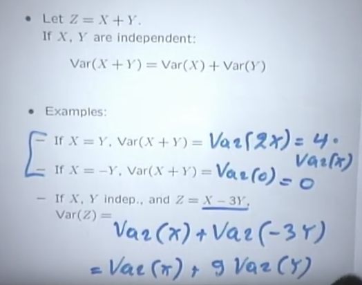
   In the example, since $X=Y$, then $X$ and $Y$ are not independent, so ..

5. Standard deviation

   $$\sigma_X=\sqrt{var(X)}$$

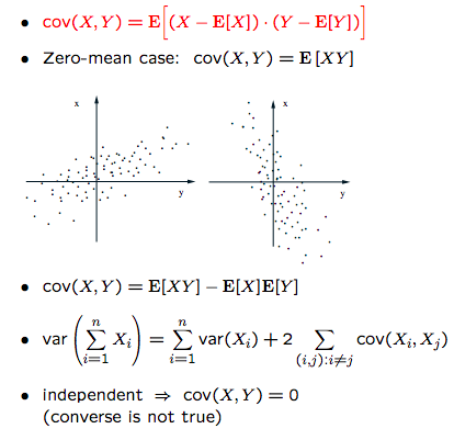
6. Covariance

   

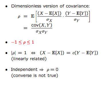
7. Correlation coefficient

   

Binomial Random Variable

1. Definition

   

   

2. Binomial mean and variance

   $X= # $ of successes in $n$ independent trials

   $X_i=\left\{\begin{align} 1& & \text{if success in trial i}\\0&&\text{otherwise}\end{align}\right.$

   • $E(X_i)=p$

     $E(X_i)=p1+(1-p)0$

   • $E(X)=np$

     $E(X)=E(x_1,x_2,…,x_n)=E(x_1)+E(x_2)+…+E(x_n)=np$

   • $Var(X_i)=p-p^2$

     $Var(X_i)=E(X_i^2)-E(X_i)^2$

     $X_i^2=\left\{\begin{align} 1& & \text{if success in trial i}\\0&&\text{otherwise}\end{align}\right.$

     So $E(X_i^2)=1p+0(1-p)=p$

     $Var(X_i)=E(X_i^2)-E(X_i)^2=p-p^2$

   • $Var(X)=n(p-p^2)$

     $Var(X)=Var(X_i,X_2,…,X_n)$

     because $X_i$ is independent to each other, so

     $Var(X)=Var(X_i,X_2,…,X_n)=Var(X_1)+Var(X_2)+…+Var(X_n)=nVar(X_i)$

3. Example-Hat Problem

   • $n$ people throw their hats in a box and then pick one at random.

     Let $X$ be the number of people who get their own hat. We want to find out $E(X)$. This is Binomial distribution:

     $X_i=\left\{\begin{align} 1& & \text{if i selects his hat}\\0&&\text{otherwise}\end{align}\right.$

   • $P(X_i)=\frac{1}{n}$

   • $E(X_i)=1\frac{1}{n}+0(1-\frac{1}{n})=\frac{1}{n}$

   • the $X_i$ are not independent

   • $E(X)=E(X_1)+E(X_2)+…+E(X_n)$ is always true no matter whether $X_i$ are independent or not.

     $E(X)=E(X_1)+E(X_2)+…+E(X_n)=n*\frac{1}{n}=1$

   • $Var(X)=E(X^2)-E(X)^2=E(X^2)-1$

     because $X$ is the number of people who has his hat, so $X=X_1+X_2+…+X_n$, then $X^2=\sum_i X_i^2+\sum_{i,j}X_iX_j$

     $Var(X)=E(X^2)-1=nE(X_i^2)+n(n-1)E(X_iX_j)-1$

     $E(X_i^2)=E(X_i)=\frac{1}{n}$

     $P(X_iX_j=1)=P(X_i=1)P(X_J=1|X_i=1)=\frac{1}{n}\frac{1}{n-1}=E(X_iX_j)$

     $Var(X)=E(X^2)-1=nE(X_i^2)+n(n-1)E(X_iX_j)-1=n\frac{1}{n}+n(n-1)\frac{1}{n}\frac{1}{n-1}-1=1$

Continuous Random Variable

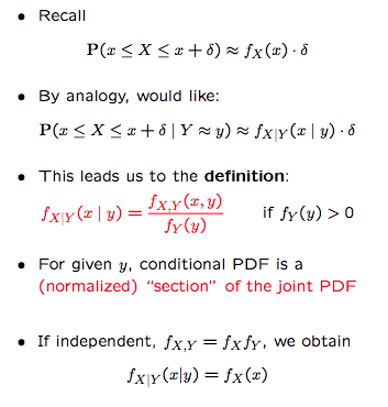
1. PDF (Probability Density Function) :

   $X$ has PDF $f(x)$ if $P(a\le{X}\le{b})=\int_{a}^{b}f(x)$

   • According to this definition, the probability of one point is 0: $P(a\le{X}\le{a})=\int_{a}^{a}f(x)=0$

   • 

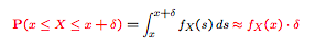
     so pdf describes the the probability of intervals.

   • n

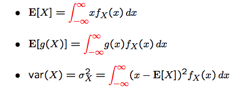
2. Means and Variances

   

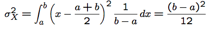
3. continuous uniform r.v.

   

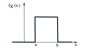
   • $f(x)=\frac{1}{b-a},a\le x \le b$
   • $E(X)=\int_{a}^{b}x\frac{x}{b-a}=\frac{a+b}{2}$
   • 

4. Cumulative distribution function(CDF)

   if $X$ has PDF $f$, then the CDF is $F(X)=P(X\le{x})=\int_{-\infty}^{x}f(t)dt$

5. Gaussian (normal) PDF

   • 

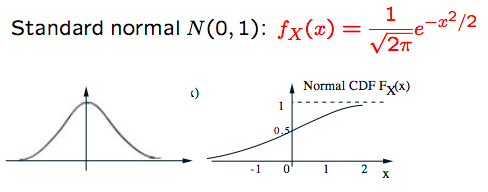
     The factor $\frac{1}{\sqrt{2\pi}}$ is to make the calculus equal 1.

     $E(X)=1, Var(X)=1$

   • 

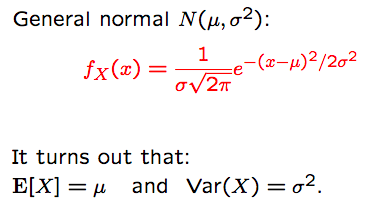
   • Let $Y=aX+b$, then

     $E(Y)=a\mu +b$, $Var(Y)=a^2 \sigma^2$

     Fact: $Y\sim N(a\mu+b,a^2\sigma^2)$, which means linear functions of normal random variabls are themselevs normal.

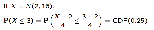
   • If $X\sim N(\mu,\sigma^2)$, then $\frac{X-\mu}{\sigma}\sim N(0,1)$

     so based on this transform, we can simplify our cdf calculation:

     

Multiple Continuous Random Variables

Joint PDF

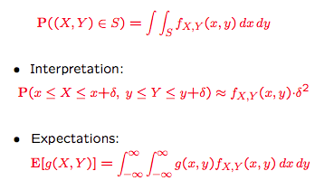
• From the joint to the marginal:

  $f_X(x)=\int_{-\infin}^{\infin}f_{X,Y}(x,y)dy$

• $X$ and $Y$ are called independent if:

  $f_{X,Y}(x,y)=f_{X}(x)f_{Y}(y)$

Buffon’s needle

1. problem setting

   

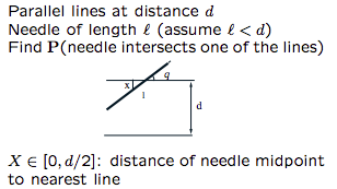
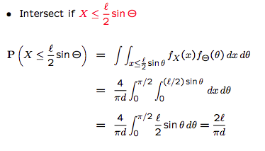
2. analysis

   $X$, $\Theta$ are uniform and independent to each other

   $f_{X,\Theta}(x,\theta)=f_X(x)f_{\Theta}(\theta)=\frac{2}{d}\frac{2}{\pi}$, where $0\le x \le \frac{d}{2}$, $0\le \theta \le\frac{\pi}{2}$

   

conditioning

Stick-breaking example

problem setting

Break a stick of length $l$ twice: break at $X$ uniformly in $[0,l]$; then break at $Y$ uniformly in $[0,X]$

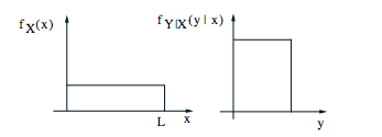
analysis

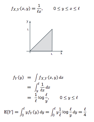
$f_{X,Y}(x,y)=f_{X}(x)f_{Y|X}(y|x)=\frac{1}{l}\frac{1}{x}$

$E(Y|X=x)=\int yf_{Y|X}(y|X=x)dy=\int_{0}^{x}y\frac{1}{x}dy=\frac{x}{2}$

Derived Distribution

Method

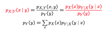
1. The discrete value bayes

   

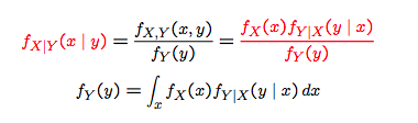
   The continuous counterpart

   

   discrete $x$ and continuous $y$

   

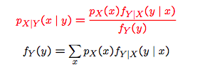
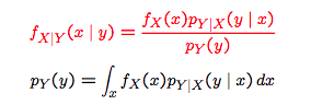
   continuous $x$ and discrete $y$

   

Examples

1. Example One

   Say $X : $ uniform on $[0,2]$. And we want to the PDF of $Y=X^3$.

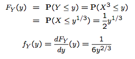
   Firstly, we calculate the PMF of $Y$, $F_Y(y)$, where $y\in[0,8]$. According to the definition of PMF,

   $$F_Y(y)=P(Y\le y)$$

   And $Y=X^3$, so we have:

   $$F_Y(y)=P(Y\le y)=P(X^3 \le y)=P(X\le y^{\frac{1}{3}})$$

   Now we want to calculate the mass probability of $X\le y^{\frac{1}{3}}$. We know that $X$ is uniform, and according to the following pic, $P(X\le y^{\frac{1}{3}})$ is the area of length=$ y^{\frac{1}{3}}$ and height=$\frac{1}{2}$

   

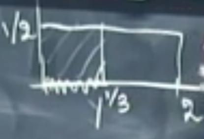
   so we have

   

2. Example Two

   Calculate the PDF of $Y=aX+b$.

   $$F_Y(y)=P(Y\le y)=P(aX+b \le y)=P(aX \le y-b)\\ F_Y(y)= \left\{ \begin{align} &P(X\le \frac{y-b}{a}) & \text{if a >=0 }\\ &P(X\ge \frac{y-b}{a})=1- P(X\le \frac{y-b}{a})&\text{if a <=0} \end{align} \right.$$

   Then the PDF is:

   $$F_Y(y)= \left\{ \begin{align} &P(X\le \frac{y-b}{a}) & \text{if a >=0 }\\ &P(X\ge \frac{y-b}{a})=1- P(X\le \frac{y-b}{a})&\text{if a <=0} \end{align} \right.$$

   Because the $P(X\le x)=F_X(x)$,

   $$F_Y(y)= \left\{ \begin{align} &F_X( \frac{y-b}{a}) & \text{if a >=0 }\\ &1- F_X( \frac{y-b}{a}) &\text{if a <=0} \end{align} \right.$$

   Then the PDF is

   $$f_Y(y)= \left\{ \begin{align} &\frac{1}{a}f_X( \frac{y-b}{a}) & \text{if a >=0 }\\ &- \frac{1}{a}f_X( \frac{y-b}{a}) &\text{if a <=0} \end{align} \right.$$

   So overall,

   $$f_Y(y)=\frac{1}{|a|}f_X( \frac{y-b}{a})$$

Bernoulli process

1. Definition

   

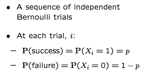
2. Properties

   There is a random process and the sequence of random variables is $X_1, X_2,…$

   $$E(X_t)=1\times p+0\times (1-p)=p\\ Var(X_t)=E(X_t^2)-E^2(X_t)=p-p^2$$

   And for the infinite sequence and no matter what the variable value is, the probability of infinite sequence is :

   $$P=P(X_1)P(X_2)...P(X_\infin)=p^k (1-p)^g\\ lim_{k\to\infin,g_\to \infin}p^k (1-p)^g=0\\ P=0$$

   Number of success $S$ in $n$ time slots

   $$P(S=k)=(_{k}^{n})p(1-p)\\ E[S]=kp\\ Var(S)=kp(1-p)$$

   Let $T_1$ be the number of trials until first success:

   $$P(T_1=t)=(1-p)^{(t-1)}p$$

   Memoryless peoperty: what happens in the past has no effect on the future random provess

   $$E[T_1]=\frac{1}p{}\\ Var(T_1)=\frac{1-p}{p^2}$$

Log

乘除 —> 加减

1. $log_a(MN)=log_a{M}+log_a{N}$
2. $log_a{\frac{M}{N}}=log_a{M}-log_a{N}$

Unbiased estimator

Additive Chernoff Bound

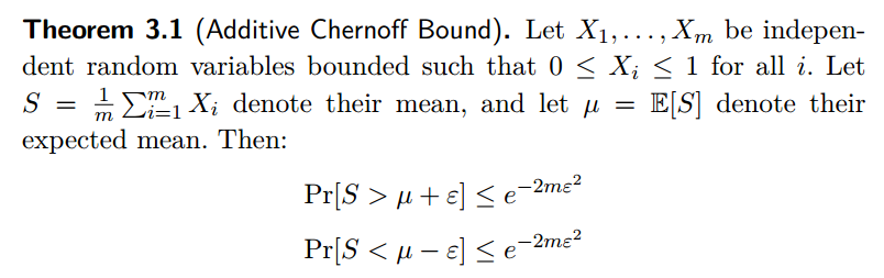
上式即

$$P(|S\ge{\mu}|\ge\epsilon)\le2e^{-2m\epsilon^2}$$

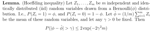
Lemma说明我们用随机变量的均值$\hat{\phi}$取估计参数$\phi$, 估计的参数和实际参数的差超过一个特定数值的概率有一确定的上界，并且随着样本量m的增大，$\hat{\phi}$越接近$\phi$.

Johnson-Lindenstrauss Lemma

The lemma states that a small set of points in a high-dimensional space can be embedded into a space of much lower dimension in such a way that distances between the points are nearly preserved.

Remarks:

1. the new dimention $n$ is decided by data sample number $m$ and error bound $\epsilon$; less error (small $\epsilon$) and more sample points require more dimensions, meaning the new dimension $n$ should not be too small;
2. Johnson–Lindenstrauss 引理表明任何高维数据集均可以被随机投影到一个较低维度的欧氏空间,同时可以控制pairwise距离的失真.