Q?
- the communication cost of $n$ users for Bassily and Smith is $log_2(n)$
- the communication cost of $n$ users for k-rr is $log_2d$
- [Optimizing Locally Differentially Private Protocols] remains : what is pure? THE protocol? BLH? Threshold $T_s$ in experiment and true/false positive?
T!
- in order to optimize ldp protocol, tends to optimize encoding step,
- using domain knowledge to elimate impossible candidates to narrow down the size of encoded input.Locally Differentially Private Heavy Hitter Identification
Local differential privacy (LDP) techniques collects randomized answers from each user, with guarantees of plausible deniability; meanwhile, the aggregator can still build accurate models and predictors by analyzing large amounts of such randomized data.
Unlike other models of differential privacy, which publish randomized aggregates but still collect the exact sensitive data, LDP avoids collecting exact personal information in the first place, thus providing a stronger assurance to the users and to the aggregator.
The well-established Laplace mechanism and exponential mechanism are no longer suitable to the local setting in which a user may have only a single element to release and laplace noise may introduce too much noise. But unlike the laplace mechanism where we can use the noisy output directly, we need to do some estimation on the randomized output to get the estimator in LDP.2016-Zhan
Development Track
Local differential privacy starts from randomized response. At first, it collects binary categorical data from clients with W-RR algorithm. Then, polybasic categorical data is considered with solutions like K-RR and K-RAPPOR methods. After that, Random Matrix Projection is proposed for dealling with extremely large categorical data in the practical setting.
Since the method above is limited to categorical data, so [Duchi et al.] proposed for numeric data and details algorithm is in [Collecting and Analyzing Data from Smart Device Users with Local Differential Privacy] and based on Duchi, harmony algorithm is developed.
The most methods above assmue that each client only has one value, so the mechanism for set-value setting is proposed [Heavy Hitter Estimation over Set-Valued Data with Local Differential Privacy].
And in real world, the collecting process in the client end happens frequently, like daily or every few hours. So methods for data collecting regularly is proposed like RAPPOR and [Collecting Telemetry Data Privately]
Recently, a mechanism for computing joint distribution of data attributes collected by LDP is proposed in [Building a RAPPOR with the Unknown- Privacy-Preserving Learning of Associations and Data Dictionaries 12.45.24 PM] and [LoPub: High-Dimensional Crowdsourced Data Publication With Local Differential Privacy]
Definition
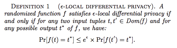
- According to the above definition, the aggregator, who receives the perturbed tuple $t*$ , cannot distinguish whether the true tuple is $t$ or another tuple $t$ with high confidence (controlled by parameter $\epsilon$), regardless of the background information of the aggregator.
- There is no neighbour databases in the local-DP; instead, for a local user, all pairs of his values should be undistinguished by using the mechanism.
- While LDP provides rigorous privacy protection in the local setting, its drawback is on the utility side. In real-world applications, where the universe size $Dom(f)$ is large, achieving a reasonable trade-off between privacy and utility under LDP is almost a chimera. For example, in location protection, $Dom(f)$ is all possible locations of a user, which could be extremely large.
Comparison With Standard DP
Standard DP
More precisely, let $M$ be a (noisy) mechanism for answering a certain query on a generic database $D$, and let $P[M(D) \in S]$ denote the probability that the answer given by $M$ to the query, on $D$, is in the (measurable) set of values $S$. We say that $M$ is $\epsilon$-differentially private if for every pairs of adjacent databases $D$ and $D’$ (i.e., differing only for the value of a single individual), and for every measurable set $S$, we have $P[M(D) \in S] ≤ e^{\epsilon}P[M(D’) \in S]$.
LDP
Technically, an obfuscation mechanism $M$ is locally differentially private with privacy level $\epsilon$ if for every pair of input values $x$, $x’$ $\in X$ (the set of possible values for the data of a generic user), and for every measurable set $S$, we have $P[M(x) \in S] ≤ e^{\epsilon} P[M(x 0 ) \in S]$. The idea is that the user provides $M(x)$ to the data collector, and not $x$.
Mechanism
Binary Values
W-RR-Categorical data
Probelm setting
In the binary attribute setting, say each user has a data $x, x\in\{0,1\}$。Now the user ranodmly sends his data $x=0 \ or \ x=1$ with a probability.
Now we want $P$ to ensure Local-DP and at the same time achieve a good utility.
Analysis
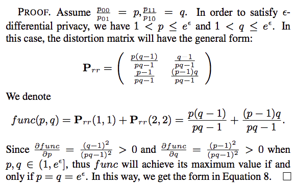
Without loss of generality, we assume the randomized response still favors the true value, i.e., $p_{00},p_{11}\gt{0.5}$;At the same time, $\frac{p_{00}}{p_{01}}\le{e^\epsilon}$ to ensure differential privacy.
Conclusion
So based on above proof, we can get the transit matrix:
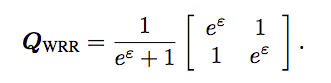
- W-RR (Warner’s randomized response model) is optimal for binary distribution minimax estimation.
- For all binary distributions $p$, all loss functions $l$, and all privacy levels $\epsilon$, $Q_{WRR}$ is the optimal solution to the private minimax distribution estimation problem.
Utility
Each user reports her true answer $t$ with probability $p$, and a random answer with probability $1 − p$. The latter has the same probability to be −1 and +1, whose expected value is zero. Therefore, the expected value for ui’s reported value is $p \times t$; thus, we can obtain an unbiased estimate of true answer by multiplying the reported value by a scaling factor $c = 1/p$.
$p_{00}=p+(1-p)*(1/2)\ \to \ p=\frac{e^\epsilon -1}{e^\epsilon +1}$.
So each user reports his random value in the following way to get an unbiased estimator:
Once the aggregator receives all reported values for attribute $t$ , it computes the average over all users, which is an estimate of the mean value $\mathbb{E}[t]$ for $t$. Since $t$ can be either $+1$ or $-1$, the the percentage of users with $+1$ is $\frac{1+\mathbb{E}[t]}{2}$ and +1 is $\frac{1-\mathbb{E}[t]}{2}$
Polychotomous Values
Problem setting
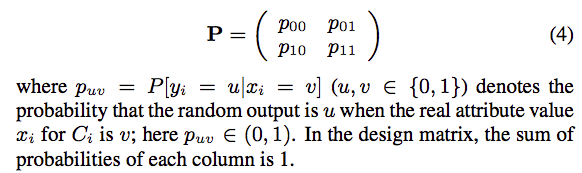
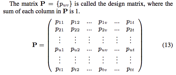
Now we extend the question to multiple attributes and each user has a data $x, x\in\{0,1,2,…,t\}$。And the transit matrix is
Solution
K-ary Randomized Response-Categorical data
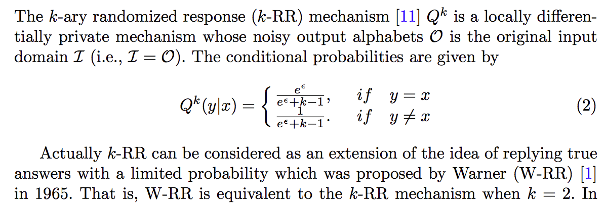
Remarks:
- k-RR mechanism is optimal in the low privacy regime while suboptimal in high privacy regime.
K-RAPPOR-Categorical data
The simplest version of RAPPOR, , called the basic one-time RAPPOR and referred to herein as k-RAPPO. There are several steps here.
data representaion
K-RAPPOR maps the input $X$ of size $k$ to an output $Y=\{0,1\}^k$ of size $2^k$.
Firstly, we map $X$ deterministically to $\widetilde{X}=R^k$, the $k$-dimensional Euclidean space, where $X=x_i \ (1\le{x_i}\le{k})$ and $\widetilde{X}=e_i\in\{0,1\}^k$. Specifically, it deterministically maps $X=x_i$ to $\widetilde{X}=e_i$, where $e_i$ is the $i$-th standard basis vector.
For example, $k=3$, and the input $X=\{x_1,x_2,x_3\}$, then $\widetilde{X}$ is $\{001,010,100\}$. And $x_1$ is represented as 1st data in $\widetilde{X}$, which is 001, $x_2$ is 2ed one 010. $x_3$ is 3rd one 100.
bit perturbation
In order to achieve $\epsilon$-locally differential privacy, we randomize the coordinates of $\widetilde{X}$ independently to obtain the private vector $Y\in\{0,1\}^k$. Formally, the $j^{th}$ coordinate of $Y$ is given by :
frequency estimation[2017-Wang]
Remarks:
- for two input, take $\{001.010,100\}$ as the example, the sensitivity is 2. Because for any two different input, the difference is 2 bits.
- using w-rr as bit perturbation method
- k-RAPPOR is a optimal privacy-preserving mechanism in high privacy regime while suboptimal in low privacy regime.
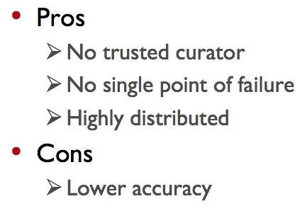
Pros:
Cons:
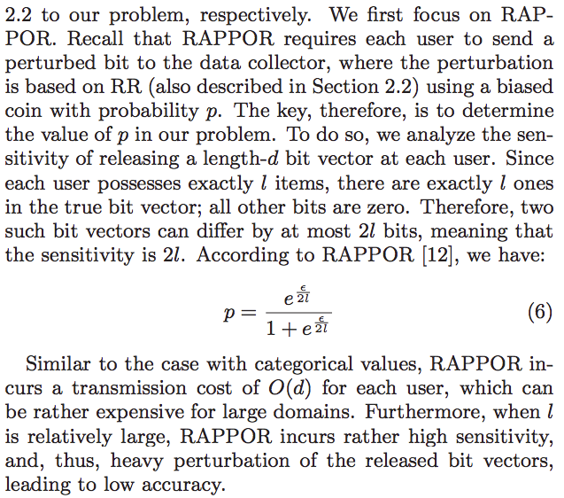
- A main drawback of RAPPOR is its high communication overhead, i.e., each user needs to transmit d bits to the data collector, which can be expensive when the number of possible items d is large.
Random Matrix Projection[2015-Bassily][2016-Chen][2017-Wang][2016-Nguyen]-Categorical data
Here, each attribute contains $k\ge2$ possible values and the aggregator aims to build a histogram that contains the estimated frequency for each of the $k$ possible values.
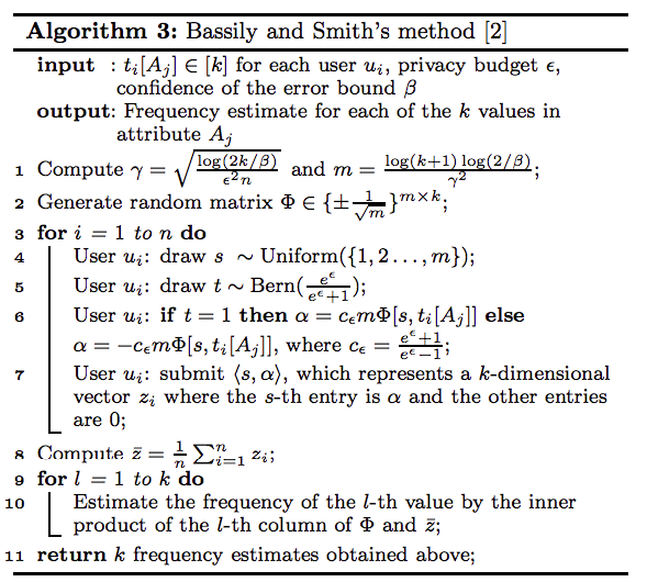
Algorithm R: $\epsilon$-Basic Randomizer
Assume that the number of possible values $d$ in the categorical attribute is far larger than the number of users $n$; hence, the method applies random projection to reduce the dimensionality from $d$ to $m$
Encoding
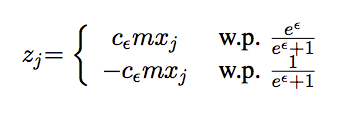
Encode($x$)=$\Phi[r,j]$, where $r$ r is selected uniformly at random from $\{1,2,…,m\}$ and $j$ is the index of $x$ in original dataset $\{x_1,x_2,…,x_d\}$.
So for each user, the return vector is $m$-dimensional vector where $s^{th} $ entry is $z_j$ and others are 0, which means the true loc in $i^{th} $ pos is maped to $s^{th}$ pos.
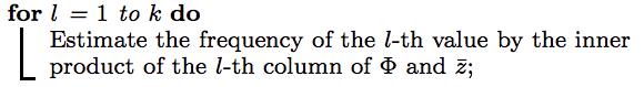
Aggregation
After receive all $z_i$ from users, we compute $\hat{z}=\frac{1}{n}\sum_{i=1}^{n}z_i$, where $\hat{z}$ is a $m$-dimentional vector.
Remarks:
- We map the input domain with size $d$ to output domain with size $m$, where $m$ is determined through Johnson-Lindenstrauss Lemma.
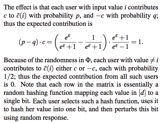
- $R$ is $\epsilon$-LDP for every choice of the index $s$
- $R(x)=z_j$ is an unbiased estimator of $x$. That is, $\mathbb{E}[R(x)]=x$
- when $d\ge n$, SH applies random projection on the data to reduce its dimensionality from d to $m = O(n)$ in a preprocessing step.
- Assuming each user only has one item.
Pros:
- the communication cost of SH between each user and the data collector is $O(1)$ rather than $O(d)$ as in RAPPOR.
Cons:
Harmony-for-numeric-Numeric data
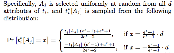
This method is to handle multiple numeric attributes. Say a user has a private tuple $t$, which contains $d$ attributes $A_1,A_2,…,A_d$. And assuming that each numeric attribute has a domain $[-1,1]$. And for numeric data, we try to calculate the mean of data.
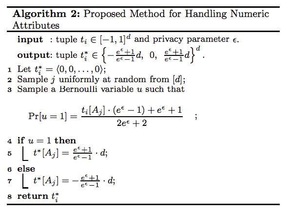
Remarks:
The return tuple $t^*_{i}$ has non-zero value on only one attribute $A_j(j\in [d])$ and this value is binary.
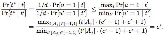
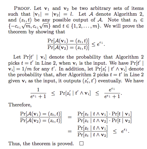
Algorithm 2 is $\epsilon$-LDP.
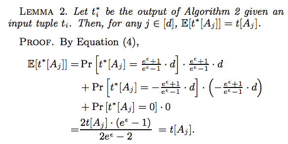
the estimator $\frac{1}{n}\sum^{n}_{i=1}t^*[A_j]$ is an unbiased estimator of the mean of $A_j$.
- xx
Summary of Mechanism
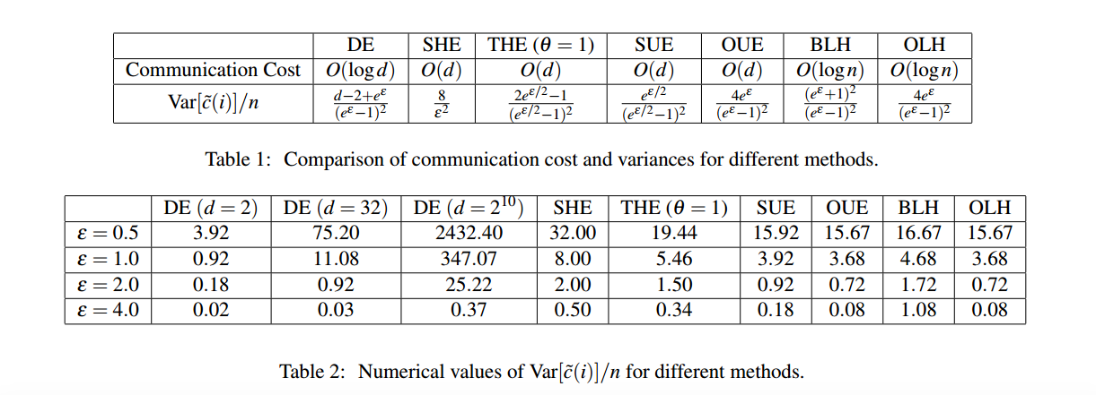
[Locally Differentially Private Protocols for Frequency Estimation] gives a comprehensive introduction of all kinds of mechanism. Here is the comparision among all methods.
Problem setting
It generalizes all methods as the same protocol. We have a input domain $x\in\{1,2,…,d\}$. For each user holding data $x_i$ and he send his data as $x_i$ with probability
$p^*$
and as others with probability as
$q^*$.
Intuitively, we want
$p^*$
to be as large as possible, and
$q^*$
to be as small as possible. However, satisfying
$\epsilon$
-LDP requires that
$\frac{p^}{q^}\le e^{\epsilon }$.
And we want to know the number of people whose data is $x_i$ and we only observe $y\in\{y_1,y_2,…y_n\}$ where $y_i$ the number of people holding data $x_i$ and is counted based on the collected samples.
Utility
Estimator
Assuming the numebr of participated users is $n$ and the true number of people holding data $x_i$ is $n_i$. For people holding $x_i$, his support to $y_i$ should be 1 and those holding other data contribute 0 to $y_i$. However, due to randomized operation, people having data $x_i$ contribute only $p^\le1$ to $y_i$ while those not holding $x_i$ contribute $q^\ge0$ to $y_i$. So for $n_i$ people who have $x_i$, the contribution to $y_i$ is $np$ while for $(n-n_i)$ people who don’t have $x_i$, their contribution to $y_i$ is $(n-n_i)q^$. So the $y_i$ can be :
since $y_i$ is known, the estimator for $n_i$ is:
and this estimator is unbiased.
To prove unbiased estimator, we need to prove $E(\hat n_i)=n_i$.
except $y_i$, all variables are constant, so
all we need to calculate is:
So, based on all above, we have
Error
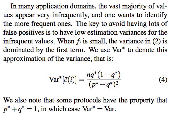
The variance of the estimator is a valuable indicator of an LDP protocol’s accuracy.
where $n_i$ is the true number of people who have data $x_i$
For each user whose data is $x_i$, his sending data process is a Bernoulli process, sending data $x_i$ if $X_{Bernoulli}=1$ with probability $p^$ and not sending $x_i$ if $X_{Bernoulli}=0$ with probability $1-p^$. So his variance contributing to $n_i$ is $p(1-p)$. For users whose data is not $x_i$, it is also a Bernoulli process and the variance is $q^(1-q^)$. So $n_i$ users contribute $n_ip^(1-p^)$ and $(n-n_i)$ users contribute $(n-n_i)q^(1-q^)$
Analysis
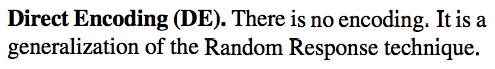
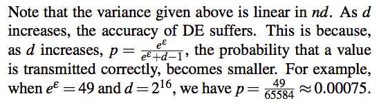
DE
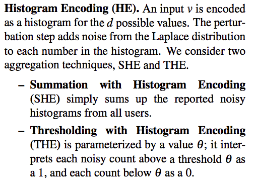
HE
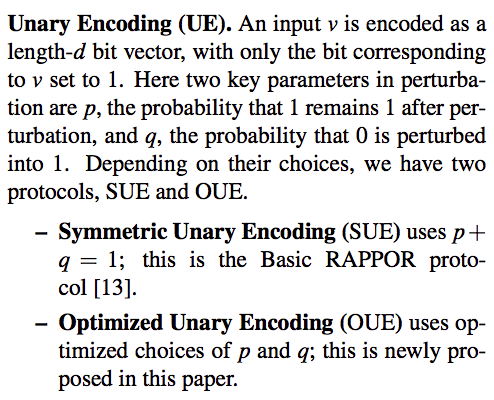
UE
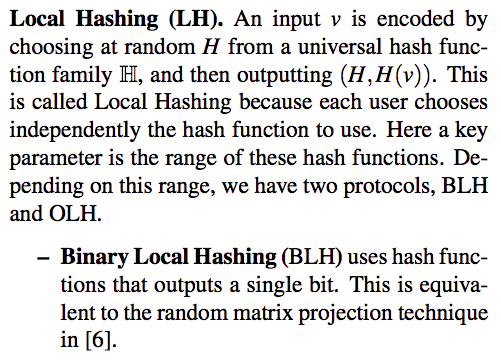
LH
Comparison
DE
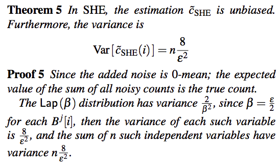
SHE
OLH||BLH
The estimator for $n_i$ is
where $d’$ is the mapping domain size.
Application
Metric-based local differential privacy[2018-Mario S. Alvim]
Heavy Hitter Estimation for Set-Valued Data[2016-Zhan]
Problem Setting
The basic LDP frequent oracle protocol enables the aggregator to estimate the frequency of any value. But when the domain of input values is large, finding the most frequent values, also known as the heavy hitters, by estimating the frequencies of all possible values, is computationally infeasible.
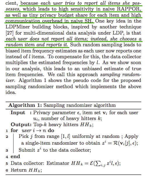
In this paper, they aims to solve the problem of heavy hitters over set-valued, where each user has a set of up to l items and they try to identify the top-k most frequent items among all users. There are $d$ items and $n$ users, and each uesr has $l$ items and try to find top-$k$ frequent items, where $k\ll\ l$ and $k\ll d$.
And each user has his own data which we call a record and every record is a set of items.
Naive solutions
Rappor for set-valued data
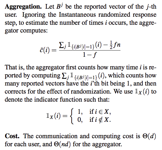
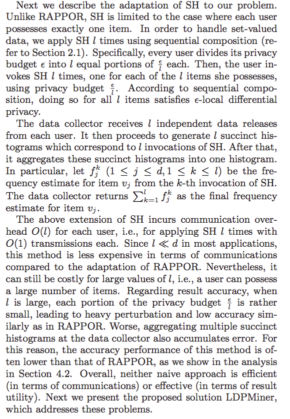
Bassily and Smith Method for set-valued data
REMARKS:
For the $\frac{\epsilon}{l}$, because each user only have a record although it has many items, we want $\epsilon$ privacy for this record. And we run algorithm $l$ times. So for overall $\epsilon$ privacy, each run should have only $\epsilon / l$ privacy budget.
Two-Phase Framework
Motivation
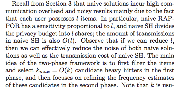
Phase I
Remarks:
Phase II
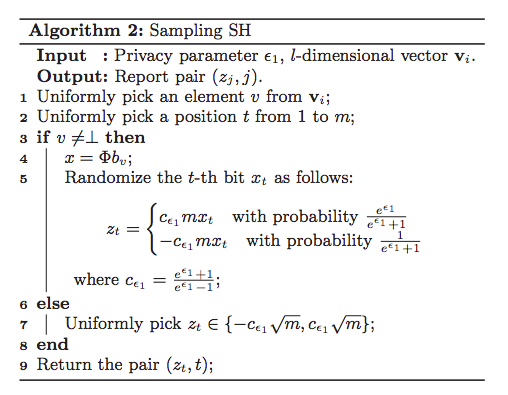
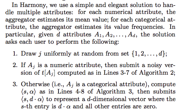
Multiple Attributes Mean or Frequencies Estimation [2016-Nguyen] [Code]
They propose the Harmony method, which can handle multiple numeric or categorical attributes.
Remarks:
- Algorithm2 is [Harmony-for-numeric] algorithm.
- Algorithm3 is [Bassily and Smith’s method]
- Each user randomly selects one attribute to submit.
Stochastic Gradient Descent
Since the gradient is the numeric number, so the author user [Harmony-for-numeric] algorithm for randomized operation. But the error by this method is $\sqrt{dlog(d)/\epsilon}$, where $d$ is the number of attributes (the length of input vector $x$).
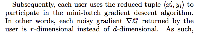
For logistic regression and SVM, they use min-batch gradient descent with the batch size $k$, reducing error to $\sqrt{dlog(d)/(\epsilon k)}$.
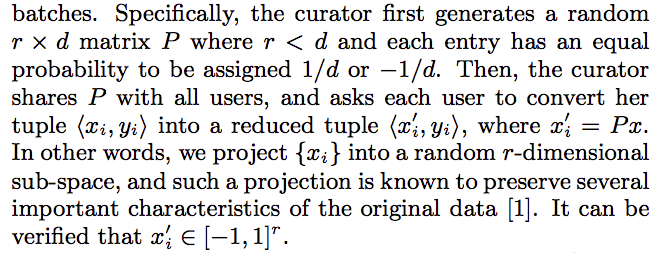
For linear regression, they introduce Dimension reduction, which introdcues error $\sqrt{rlog(r)/(\epsilon k)}$
Locations Density Estimation [2018-Kim]
A number of studies have recently been made on discrete distribution estimation in the local model, in which users obfuscate their personal data (e.g., location, response in a survey) by themselves and a data collector estimates a distribution of the original personal data from the obfuscated data.
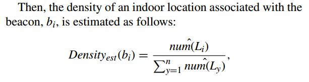
The purpose of this research is to approximately compute the distribution of users in the indoor space.
Pricacy model
data representation
There are $n$ locations $B=\{b_1,b_2,…,b_n\}$, and the location of a user is in the form of a $n$-bit array, denoted as $L$, where the bit corresponding to the user’s location is set to 1 while the others are set to 0. So the input space size is $n$, the output space size is $2^n$.
RAPPOR
The next step is to perturb L, where each bit in L is first perturbed by randomized response as follows:
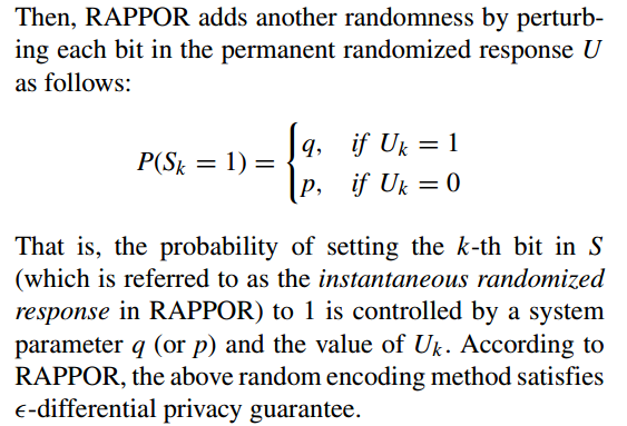
The instantaneous randomized response, S, is transmitted to the data collector server.
Estimation
STATISTIC-BASED APPROACH
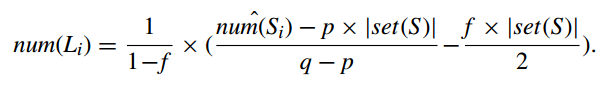
the number of the instantaneous randomized responses of which the i-th bit is expected to be set to 1, $num(S_i)$, is estimated as follows:
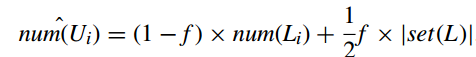
$num(U_i)$ is estimated as follows:
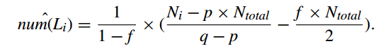
then the number of location i where users have been to can be calculated by combining above two formulas:
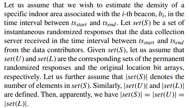
Let $N_i$ denotes the total number of instantaneous randomized responses, S, of which the i-bit is set to 1 as well as which is received between $ts_{start}$ and $ts_{end}$. And $N_{total}$ denotes the total number of instantaneous randomized responses, S, that the data collection server received from the data contributors in the time interval between $ts_{start}$ and $ts_{end}$.

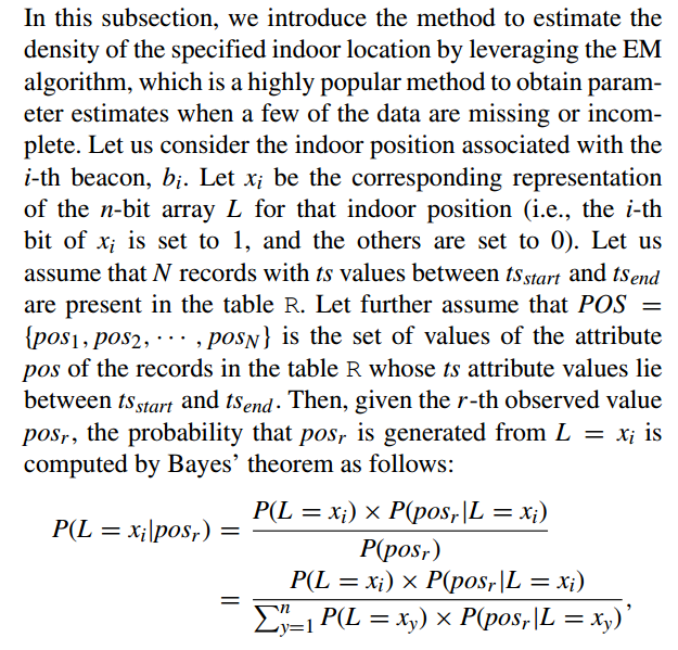
EM-BASED APPROACH
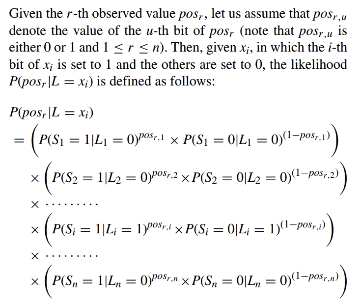
Here we intend to estimate $P(L=x_i)$.
Then we want to calculate $P(pos_r|L=x_y)$
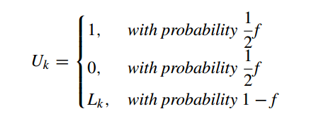
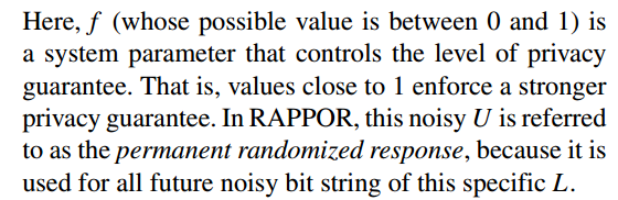
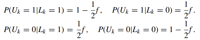
Given a $n$-bit array $L$, the probabilities that the k-th bit of the corresponding permanent randomized response, U, sets to 1 and 0 are respectively computed as follows:
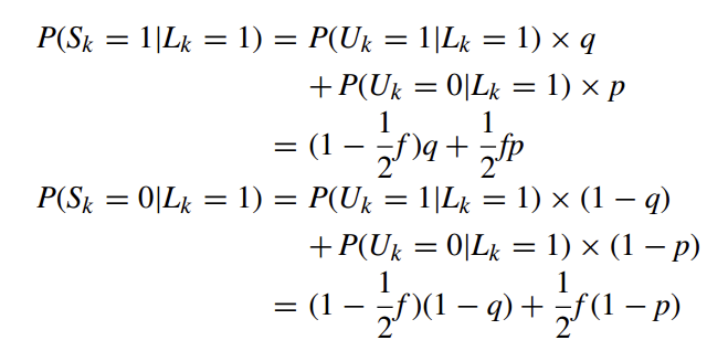
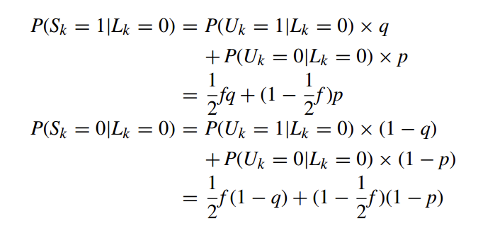
Then, Given $L_k=1$, the probabilities that the k-th bit of the instantaneous randomized response, S, sets to 1 and 0 are respectively computed as follows:
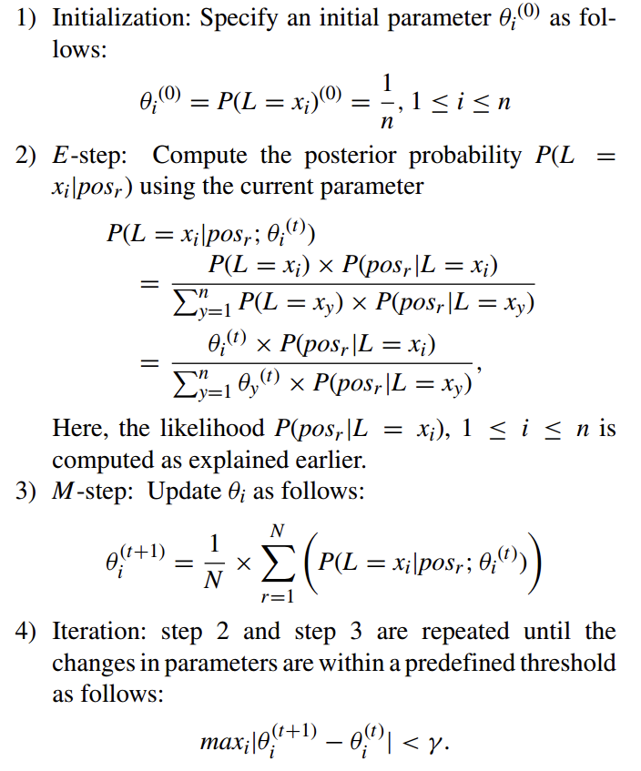
The EM algorithm that computes $P(L = x_i)$, 1 ≤ i ≤ n proceeds as follows:
Reference
[2018-Kim] Application of Local Differential Privacy to Collection of Indoor Positioning Data
[2016-Peter] Discrete Distribution Estimation under Local Privacy
[2015-Bassily] Local, Private, Efficient Protocols for Succinct Histograms
[2016-Chen] Private Spatial Data Aggregation in the Local Setting
[2017-Wang] Optimizing Locally Differentially Private Protocols
[2016-Nguyen] Collecting and Analyzing Data from Smart Device Users with Local Differential Privacy
[2016-Zhan] Heavy Hitter Estimation over Set-Valued Data with Local Differential Privacy
[2017-PPT] Local differential privacy
[2018-Mario S. Alvim] Metric-based local differential privacy for statistical applications