本文参考了1
通用学习模式
|
|
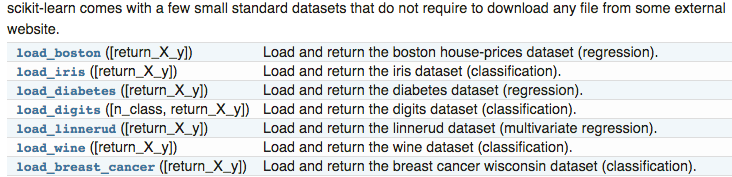
Sklearn中数据集
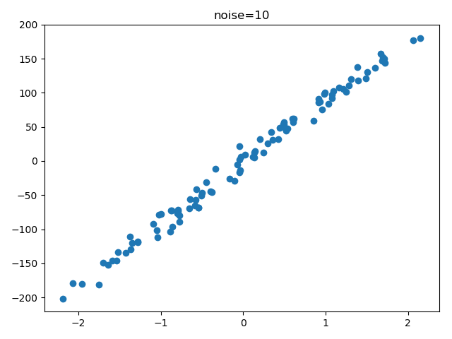
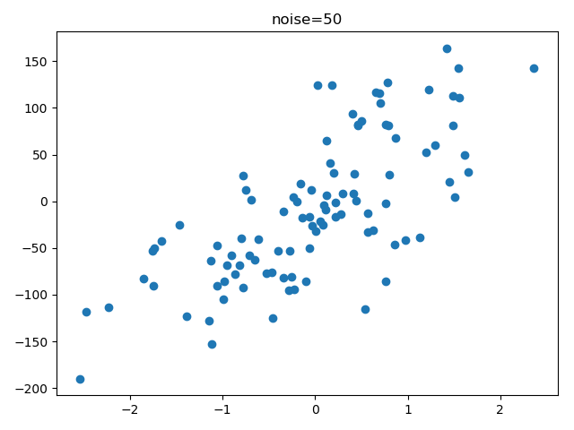
生成样本数据,按照函数的形式,输入 sample,feature,target 的个数等等
|
|
Example: 房价预测
|
|
Example:生成样本数据
|
|
Sklearn常用属性和功能
以LinearRegression方法为例
导入:包、数据和模型
12345678from sklearn import datasetsfrom sklearn.linear_model import LinearRegressionloaded_data = datasets.load_boston()data_X = loaded_data.datadata_y = loaded_data.targetmodel = LinearRegression()模型训练与预测
123model.fit(data_X, data_y)print(model.predict(data_X[:4, :]))模型参数
模型:$f(x) = w_1x_1+w_2x_2+…+x_nw_n+w_0$
model.coef_和model.intercept_属于 Model 的属性model.coef_:模型权重,$(w_1,w_2,…,w_n)$model.intercept_:$w_0$1234567891011print(model.coef_)print(model.intercept_)"""[ -1.07170557e-01 4.63952195e-02 2.08602395e-02 2.68856140e+00-1.77957587e+01 3.80475246e+00 7.51061703e-04 -1.47575880e+003.05655038e-01 -1.23293463e-02 -9.53463555e-01 9.39251272e-03-5.25466633e-01]36.4911032804"""预测效果评分
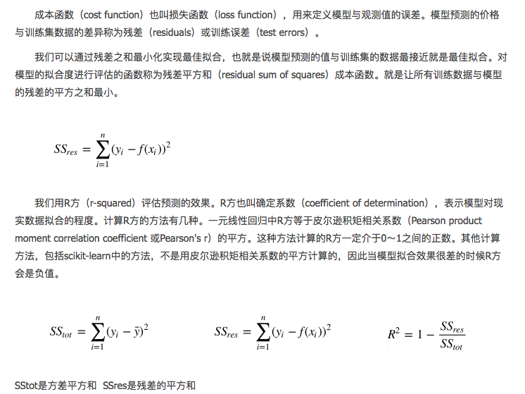
12345print(model.score(data_X, data_y)) # R^2 coefficient of determination"""0.740607742865"""$R^2$计算方法:
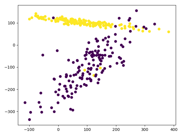
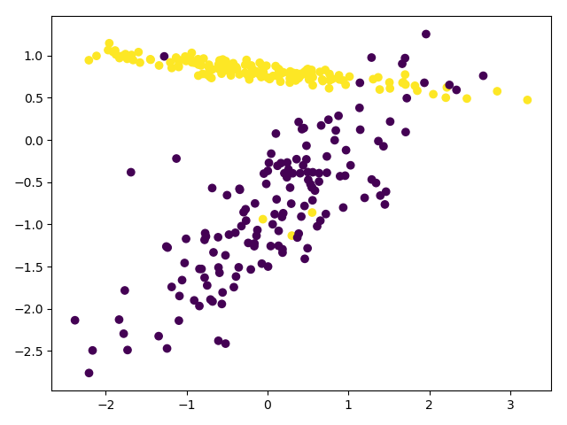
正则化
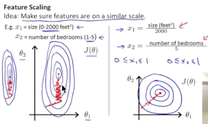
sklearn中模块preprocessing提供了scale功能。
|
|
|
|
|
|
|
|
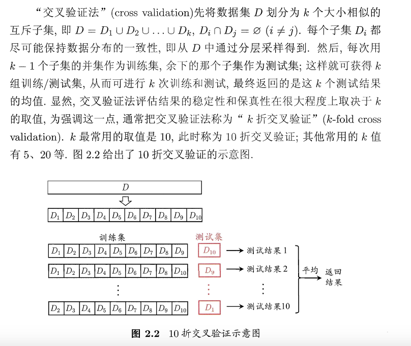
交叉验证cross-validation
|
|
有一个问题,k次训练会得到k个模型,也就是说每个模型的系数可能都不相同,那最终的模型是如何得到的呢?这个问题困扰了我很久。今天,通过阅读网上资料和matlab源码,解决这个问题,其实原理很简单。交叉验证只是一种模型验证方法,而不是一个模型优化方法,即用于评估一种模型在实际情况下的预测能力。比如,现在有若干个分类模型(决策树、SVM、KNN等),通过k-fold cross validation,可得到不同模型的误差值,进而选择最合适的模型,但是无法确定每个模型中的最优参数。
|
|
|
|
|
|
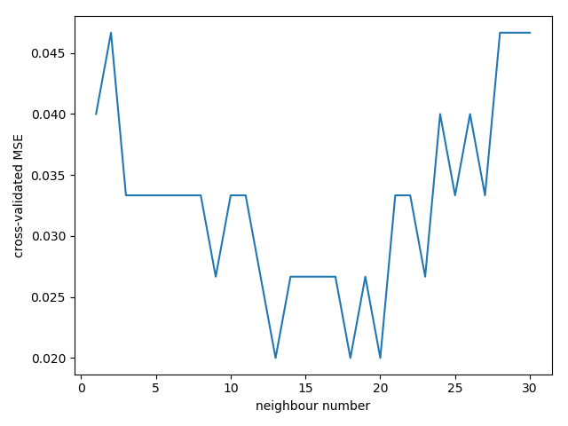
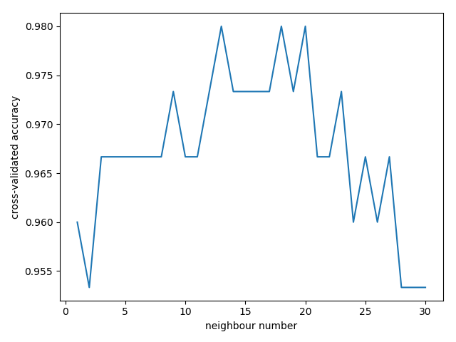
一般来说
准确率(accuracy)会用于判断分类(Classification)模型的好坏。
平均方差(Mean squared error)会用于判断回归(Regression)模型的好坏。
Overfitting
overfitting检查
1234567891011121314151617181920212223242526from sklearn.model_selection import learning_curvefrom sklearn.datasets import load_digitsfrom sklearn.svm import SVCimport matplotlib.pyplot as pltimport numpy as npdigits = load_digits()x = digits.datay = digits.targettrain_sizes,train_loss,test_loss = learning_curve(SVC(gamma=0.001),x,y,cv=10,scoring='mean_squared_error',train_sizes=[0.1,0.25,0.5,0.75,1])train_loss_mean = -np.mean(train_loss,axis=1)test_loss_mean = -np.mean(test_loss,axis=1)plt.plot(train_sizes, train_loss_mean, 'o-', color="r",label="Training")plt.plot(train_sizes, test_loss_mean, 'o-', color="g",label="Cross-validation")plt.xlabel("Training examples")plt.ylabel("Loss")plt.legend(loc="best")plt.show()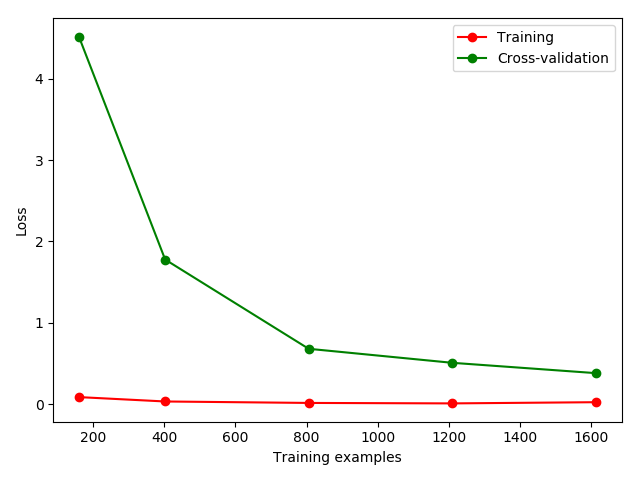
- 加载digits数据集,其包含的是手写体的数字,从0到9。数据集总共有1797个样本,每个样本由64个特征组成, 分别为其手写体对应的8×8像素表示,每个特征取值0~16。
- 采用K折交叉验证
cv=10, 选择平均方差检视模型效能scoring='mean_squared_error', 样本由小到大分成5轮检视学习曲线(10%, 25%, 50%, 75%, 100%) - 从图中可以看出,随着训练样本的变大,训练误差和测试误差同时变小,说明模型的准确度因为样本增多而增高;
这次我们来验证
SVC中的一个参数gamma在什么范围内能使 model 产生好的结果. 以及过拟合和gamma取值的关系.12345678910111213141516171819202122232425262728from sklearn.model_selection import validation_curvefrom sklearn.datasets import load_digitsfrom sklearn.svm import SVCimport matplotlib.pyplot as pltimport numpy as npdigits = load_digits()x = digits.datay = digits.targetparam_range = np.logspace(-6,-2.3,5)train_loss,test_loss = validation_curve(SVC(),x,y,param_name='gamma',param_range=param_range,cv=10,scoring='mean_squared_error')train_loss_mean = -np.mean(train_loss,axis=1)test_loss_mean = -np.mean(test_loss,axis=1)plt.plot(param_range, train_loss_mean, 'o-', color="r",label="Training")plt.plot(param_range, test_loss_mean, 'o-', color="g",label="Cross-validation")plt.xlabel("gamma")plt.ylabel("Loss")plt.legend(loc="best")plt.show()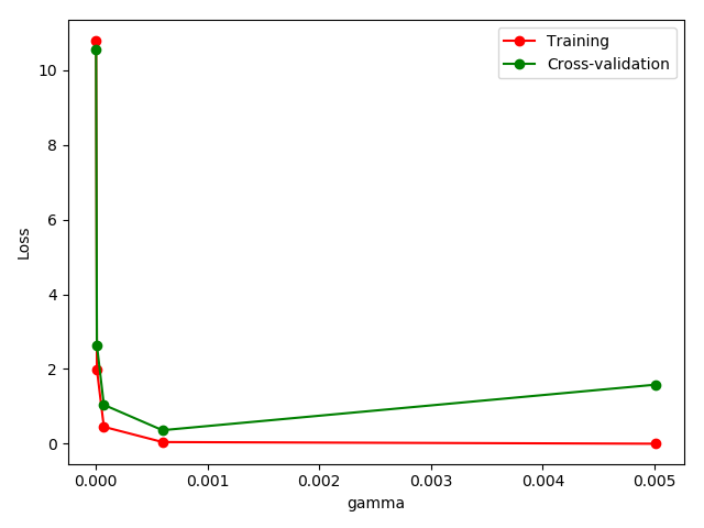
从图中可以看到,当gamma从0到0.0005左右,training error和test error都在减小,说明模型效果随着gamma的最大而变好;但是当gamma继续增大,test error 却开始增加,说明gamma大于0.001时模型过拟合了。
模型保存
pickle
123456789101112131415161718192021from sklearn import svmfrom sklearn import datasetsclf = svm.SVC()iris = datasets.load_iris()X, y = iris.data, iris.targetclf.fit(X,y)import pickle #pickle模块#保存Model(注:save文件夹要预先建立,否则会报错)with open('save/clf.pickle', 'wb') as f:pickle.dump(clf, f)#读取Modelwith open('save/clf.pickle', 'rb') as f:clf2 = pickle.load(f)#测试读取后的Modelprint(clf2.predict(X[0:1]))# [0]joblib
123456789101112from sklearn.externals import joblib #jbolib模块#保存Model(注:save文件夹要预先建立,否则会报错)joblib.dump(clf, 'save/clf.pkl')#读取Modelclf3 = joblib.load('save/clf.pkl')#测试读取后的Modelprint(clf3.predict(X[0:1]))# [0]