ML - K-Nearest Neighbors

How kNN algorithm works

k nearest neighbor (kNN): how it works

How K-Nearest Neighbors (kNN) Classifier Works

kNN (k-Nearest Neighbors) is a classification algorithm. It is a simple algorithm that stores all available cases and classifies new cases based on a similarity measure (e.g., distance functions).

Algorithm

For a new case to be classified, we calculate the distance between this case and each training sample. And we rank the distance in an ascending way and pick the top-k samples with smallest distance with the new case as its k-nearest neighbour. And this case is classified by a majority vote of its neighbors, with the case being assigned to the class most common amongst its K nearest neighbors. If K = 1, then the case is simply assigned to the class of its nearest neighbor.

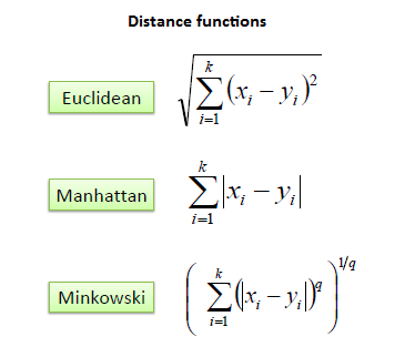
distance

It should also be noted that all three distance measures are valid for continuous variables. In the instance of categorical variables the Hamming distance must be used.

Say we have a categorical attribute gender and its domain is $\{male, female\}$. And for a new case $x$ and its gender is $male$. For all the training sample, we calculate the gender distance between each sample and the new case. If their gender is same, then the distance is 0; else the distance is 1.

normalization

Because the distance of categorical attribute is either 0 or 1, standardization of the numerical variables between 0 and 1 is needed when there is a mixture of numerical and categorical variables in the dataset.

K choice

Choosing the optimal value for K is best done by first inspecting the data. In general, a large K value is more precise as it reduces the overall noise but there is no guarantee. Cross-validation is another way to retrospectively determine a good K value by using an independent dataset to validate the K value. Historically, the optimal K for most datasets has been between 3-10. That produces much better results than 1NN.

Example1

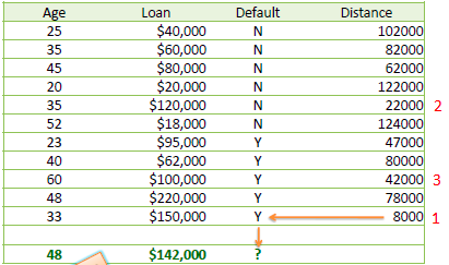
Say we have the training sample database concerning credit default as follows, Age and Loan are two numerical variables (predictors) and Default is the target.

Age	Loan	Default
25	$40,000	N
35	$60,000	N
45	$80,000	N
20	$20,000	N
35	$120,000	N
52	$18,000	N
23	$95,000	Y
40	$62,000	Y
60	$100,000	Y
48	$220,000	Y
33	$150,000	Y

Now we have an unknown case (Age=48 and Loan=$142,000). And we want to predict the credit default for this case using Euclidean distance. So using the following formula to calculate the distance:

$$d =\sqrt{(x_1-y_1)^2+(x_2-y_2)^2}$$

We can get the following:

With k=3, there are two Default=Y and one Default=N out of the three closest neighbors. So the prediction for this case is Default=Y.

Example2

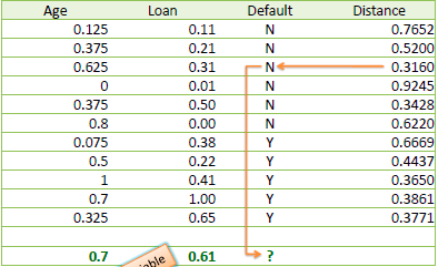
One major drawback in calculating distance measures directly from the training set is in the case where variables have different measurement scales or there is a mixture of numerical and categorical variables. For example, if one variable is based on annual income in dollars, and the other is based on age in years then income will have a much higher influence on the distance calculated. One solution is to standardize the training set as shown below.

$$X_s=\frac{X-X_{min}}{X_{max}-X_{min}}$$

Implementation

import numpy as np
from collections import Counter

class KNearestNeighbor():

    def train(self,X,y):
        self.X_train = X
        self.y_train = y

    def compute_distances_two_loops(self, X):
        num_test = X.shape[0]
        num_train = self.X_train.shape[0]
        dists = np.zeros((num_test, num_train))
        for i in range(num_test):
            for j in range(num_train):
                dists[i, j] = np.linalg.norm(X[i] - self.X_train[j])
        return dists

    def compute_distances_one_loop(self, X):
        num_test = X.shape[0]
        num_train = self.X_train.shape[0]
        dists = np.zeros((num_test, num_train))
        for i in range(num_test):
            dists[i] = np.linalg.norm(X[i] - self.X_train, axis=1)
        return dists

    def compute_distances_no_loops(self, X):
        num_test = X.shape[0]
        num_train = self.X_train.shape[0]
        dists = np.zeros((num_test, num_train))
        # https://medium.com/dataholiks-distillery/l2-distance-matrix-vectorization-trick-26aa3247ac6c
        x = np.sum(X ** 2, axis=1).reshape(num_test, 1)  # shape = (num_test,1)
        y = np.sum(self.X_train ** 2, axis=1)  # shape = (1,num_train)
        xy = np.dot(X, self.X_train.T)
        dists = np.sqrt(x + y - 2 * xy)  # shape of (x+y) = (num_test,num_train)
        return dists

    def predict_labels(self, dists, k=1):
        num_test = dists.shape[0]
        y_pred = np.zeros(num_test)
        for i in range(num_test):
            closest_y = []
            dist = dists[i, :]
            idx = np.argsort(dist)[:k]  # choose least distance
            closest_y = self.y_train[idx]
            b = Counter(sorted(closest_y))
            c = b.most_common(1)[0][0]
            y_pred[i] = c
        return y_pred

    def predict(self, X, k=1, num_loops=0):
        if num_loops == 0:
            dists = self.compute_distances_no_loops(X)
        elif num_loops == 1:
            dists = self.compute_distances_one_loop(X)
        elif num_loops == 2:
            dists = self.compute_distances_two_loops(X)
        else:
            raise ValueError('Invalid value %d for num_loops' % num_loops)

        return self.predict_labels(dists, k=k)


if __name__ == '__main__':
    X_train = []
    y_train = []

    classifier = KNearestNeighbor()

    num_folds = 5
    k_choices = [1, 3, 5, 8, 10, 12, 15, 20, 50, 100]

    X_train_folds = np.array_split(X_train, num_folds)
    y_train_folds = np.array_split(y_train, num_folds)

    k_to_accuracies = {}

    for k in k_choices:
        accuracy = []
        for f in range(num_folds):
            xtrain = np.concatenate((X_train_folds[:f] + X_train_folds[f + 1:]), axis=0)  # have to use '+'
            ytrain = np.concatenate((y_train_folds[:f] + y_train_folds[f + 1:]), axis=0)
            xval = X_train_folds[f]
            yval = y_train_folds[f]

            num_val = len(xval)

            classifier.train(xtrain, ytrain)
            y_predict = classifier.predict(xval, k)

            num_correct = np.sum(y_predict == yval)
            accuracy.append(float(num_correct) / num_val)
        k_to_accuracies[k] = accuracy

    # *****END OF YOUR CODE (DO NOT DELETE/MODIFY THIS LINE)*****

    # Print out the computed accuracies
    for k in sorted(k_to_accuracies):
        for accuracy in k_to_accuracies[k]:
            print('k = %d, accuracy = %f' % (k, accuracy))