Experiment-Metric

箱线图

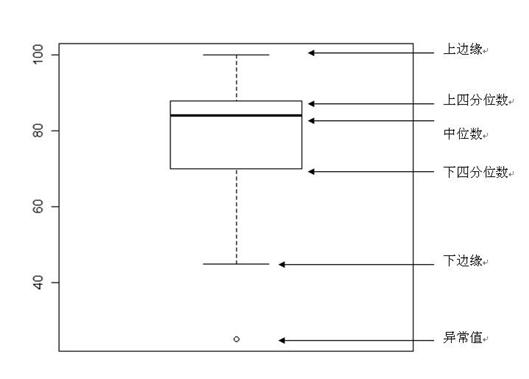
箱线图（Boxplot）也称箱须图（Box-whisker Plot），可以用于异常值检测。它是用一组数据中的最小值、第一四分位数、中位数、第三四分位数和最大值来反映数据分布的中心位置和散布范围，可以粗略地看出数据是否具有对称性。通过将多组数据的箱线图画在同一坐标上，则可以清晰地显示各组数据的分布差异，为发现问题、改进流程提供线索。

四分位数

所谓四分位数，就是把组中所有数据由小到大排列并分成四等份，处于三个分割点位置的数字就是四分位数。

• 第一四分位数（Q1），又称“较小四分位数”或“下四分位数”，等于该样本中所有数值由小到大排列后第25%的数字。
• 第二四分位数（Q2），又称“中位数”，等于该样本中所有数值由小到大排列后第50%的数字。
• 第三四分位数（Q3），又称“较大四分位数”或“上四分位数”，等于该样本中所有数值由小到大排列后第75%的数字。
• 第三四分位数与第一四分位数的差距又称四分位间距（InterQuartile Range，IQR）。

四分位数计算

1. 确定Q1、Q2、Q3的位置（n表示数字的总个数）

   • Q1的位置=（n+1）/4
   • Q2的位置=（n+1）/2
   • Q3的位置=3（n+1）/4

   对于数字个数为奇数的，其四分位数比较容易确定。例如，数字“5、47、48、15、42、41、7、39、45、40、35”共有11项，由小到大排列的结果为“5、7、15、35、39、40、41、42、45、47、48”，计算结果如下：

   • Q1的位置=（11+1）/4=3，该位置的数字是15。
   • Q2的位置=（11+1）/2=6，该位置的数字是40。
   • Q3的位置=3（11+1）/4=9，该位置的数字是45。

   而对于数字个数为偶数的，其四分位数确定起来稍微繁琐一点。例如，数字“8、17、38、39、42、44”共有6项，位置计算结果如下：

   • Q1的位置=（6+1）/4=1.75
   • Q2的位置=（6+1）/2=3.5
   • Q3的位置=3（6+1）/4=5.25

   这时的数字以数据连续为前提，由所确定位置的前后两个数字共同确定。例如，Q2的位置为3.5，则由第3个数字38和第4个数字39共同确定，计算方法是：38+（39-38）×3.5的小数部分，即38+1×0.5=38.5。该结果实际上是38和39的平均数。

   同理，Q1、Q3的计算结果如下：

   • Q1 = 8+（17-8）×0.75=14.75
   • Q3 = 42+（44-42）×0.25=42.5

MAE vs MSE

ref1

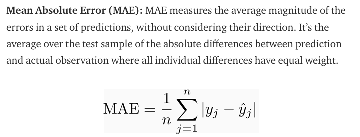
MAE(Mean Absolute Error)

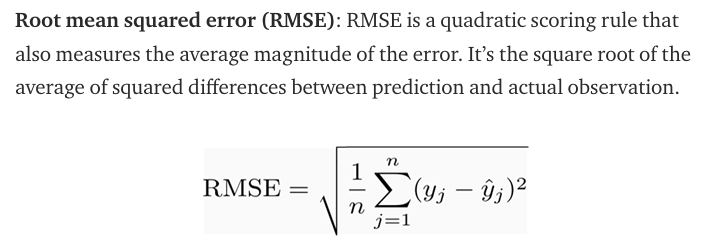
MSE(Mean Squared Error)

Comparison

1. They are both used in crowd counting as evaluation metric.

2. Roughly speaking, MAE indicates the accuracy of the estimates, and MSE indicates the robustness of the estimates.

   This is because for mse, the errors are squared before they are averaged, the MSE gives a relatively high weight to large errors. This means the RMSE should be more useful when large errors are particularly undesirable.

Confusion Matrix

A confusion matrix is a technique used for summarizing the performance of a classification algorithm i.e. it has binary outputs. Example for a classification algorithm: Predicting if the patient has cancer. Here, there can only be two outputs i.e. Yes or No.

A confusion matrix gives us a better idea of what our classification model is predicting right and what types of errors it is making.

Below is what an Confusion Matrix looks like:

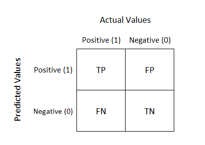
True Positive: You predicted positive and your are right.

True Negative: You predicted negative and your are right.

False Positive: (Type 1 Error): You predicted positive and you are wrong.

False Negative: (Type 2 Error): You predicted negative and you are wrong.

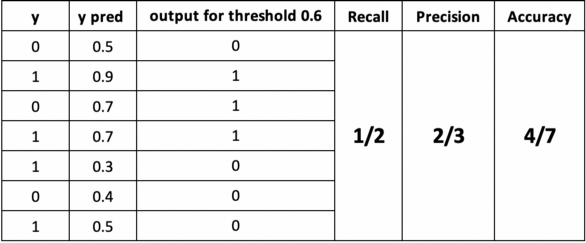
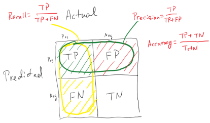
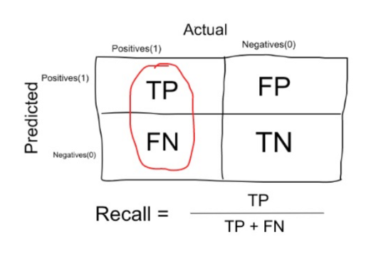
Recall

Among the data with label 1, what is the percentage of them predicted as 1?

$$\operatorname{Recall}=\frac{\mathrm{TP}}{\mathrm{TP}+\mathrm{FN}}$$

Precision

Among the data predicted as 1, what is the percenatge of correctness?

$$\text { Precision }=\frac{\mathrm{TP}}{\mathrm{TP}+\mathrm{FP}}$$

F-measure

$$F-\text {measure}=\frac{2 * \text { Recall * Precision }}{\text { Recall }+\text { Precision }}$$

accuracy常用于分类，比对两个向量，一个是真实向量，一个是预测向量，预测正确加1，最终sum除以向量长度就是准确率。

精确率(precision)的公式是katex is not defined,它计算的是所有”正确被检索的item(TP)”占所有”实际被检索到的(TP+FP)”的比例.（在所有找对找错里面，找对的概率）

召回率(recall)的公式是katex is not defined,它计算的是所有”正确被检索的item(TP)”占所有”应该检索到的item(TP+FN)”的比例。（找到正确的，能覆盖目标的所有的概率）

假如某个班级有男生80人,女生20人,共计100人.目标是找出所有女生. 现在某人挑选出50个人,其中20人是女生,另外还错误的把30个男生也当作女生挑选出来了. 作为评估者的你需要来评估(evaluation)下他的工作。

• 很容易，我们可以得到:他把其中70(20女+50男)人判定正确了,而总人数是100人，所以它的accuracy就是70 %(70 / 100).
• 在例子中就是希望知道此君得到的所有人中,正确的人(也就是女生)占有的比例.所以其precision也就是40%(20女生/(20女生+30误判为女生的男生)).
• 在例子中就是希望知道此君得到的女生占本班中所有女生的比例,所以其recall也就是100%(20女生/(20女生+ 0 误判为男生的女生))

AUC ROC Curve

What is ROC?

ROC (Receiver Operating Characteristic) Curve tells us about how good the model can distinguish between two things (e.g If a patient has a disease or no). Better models can accurately distinguish between the two. Whereas, a poor model will have difficulties in distinguishing between the two.

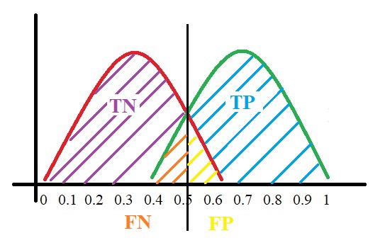
Let’s assume we have a model which predicts whether the patient has a particular disease or no. The model predicts probabilities for each patient (in python we use the“ predict_proba*” function*). Using these probabilities, we plot the distribution as shown below:

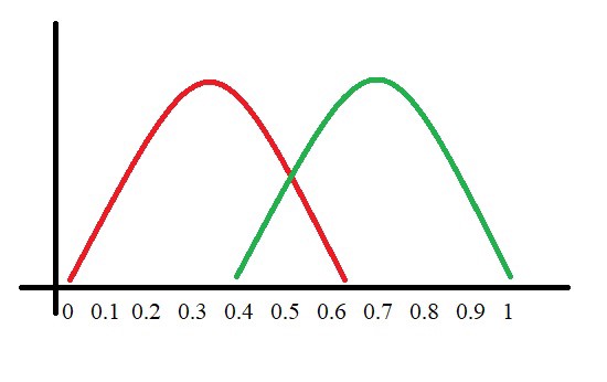
Here, the red distribution represents all the patients who do not have the disease and the green distribution represents all the patients who have the disease.

Now we got to pick a value where we need to set the cut off i.e. a threshold value, above which we will predict everyone as positive (they have the disease) and below which will predict as negative (they do not have the disease). We will set the threshold at “0.5” as shown below:

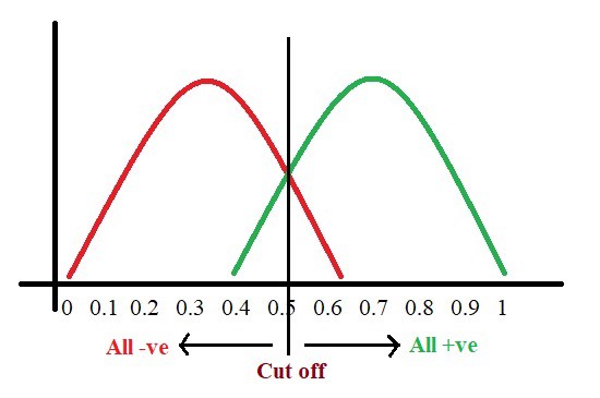
All the positive values above the threshold will be “True Positives” and the negative values above the threshold will be “False Positives” as they are predicted incorrectly as positives.

All the negative values below the threshold will be “True Negatives” and the positive values below the threshold will be “False Negative” as they are predicted incorrectly as negatives.

Here, we have got a basic idea of the model predicting correct and incorrect values with respect to the threshold set. Before we move on, let’s go through two important terms: Sensitivity and Specificity.

What is Sensitivity and Specificity?

In simple terms, the proportion of patients that were identified correctly to have the disease (i.e. True Positive) upon the total number of patients who actually have the disease is called as Sensitivity or Recall.

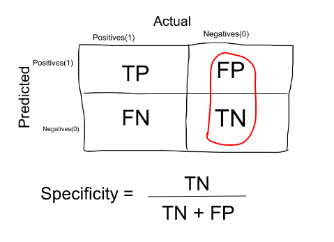
Similarly, the proportion of patients that were identified correctly to not have the disease (i.e. True Negative) upon the total number of patients who do not have the disease is called as Specificity.

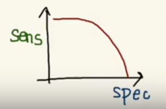
Trade-off between Sensitivity and Specificity

When we decrease the threshold, we get more positive values thus increasing the sensitivity. Meanwhile, this will decrease the specificity.

Similarly, when we increase the threshold, we get more negative values thus increasing the specificity and decreasing sensitivity.

As Sensitivity ⬇️ Specificity ⬆️

As Specificity ⬇️ Sensitivity ⬆️

But, this is not how we graph the ROC curve. To plot ROC curve, instead of Specificity we use (1 — Specificity) and the graph will look something like this:

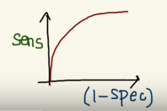
So now, when the sensitivity increases, (1 — specificity) will also increase. This curve is known as the ROC curve.

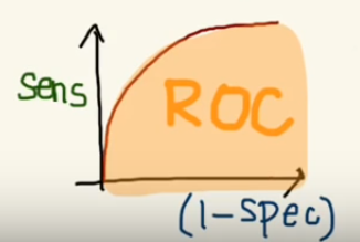
Area Under the Curve

The AUC is the area under the ROC curve. This score gives us a good idea of how well the model performances.

Let’s take a few examples

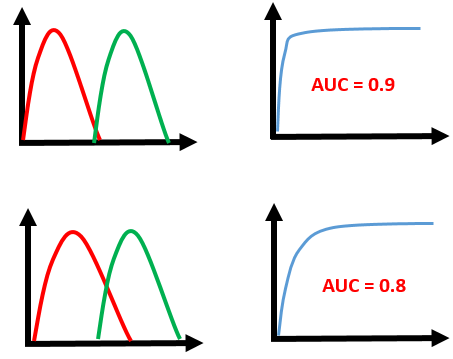
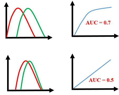
As we see, the first model does quite a good job of distinguishing the positive and the negative values. Therefore, there the AUC score is 0.9 as the area under the ROC curve is large.

Whereas, if we see the last model, predictions are completely overlapping each other and we get the AUC score of 0.5. This means that the model is performing poorly and it is predictions are almost random.

Why do we use (1 — Specificity)?

Let’s derive what exactly is (1 — Specificity):

$$\begin{array}{c}{\text { Specificity }=\frac{T N}{T N+F P}} \\ {1-\text {Specificity}=1-\frac{T N}{T N+F P}} \\ {1-\text {Specificity}=\frac{T N+F P-T N}{T N+F P}} \\ {1-\text {Specificity}=\frac{F P}{T N+F P}}\end{array}$$

As we see above, Specificity gives us the True Negative Rate and (1 — Specificity) gives us the False Positive Rate.

So the sensitivity can be called as the “True Positive Rate” and (1 — Specificity) can be called as the “False Positive Rate”.

So now we are just looking at the positives. As we increase the threshold, we decrease the TPR as well as the FPR and when we decrease the threshold, we are increasing the TPR and FPR.

Thus, AUC ROC indicates how well the probabilities from the positive classes are separated from the negative classes.

ref1

AOC是衡量一个模型是否有效的参数，比如：我们使用了grid search来暴力寻找最佳的超参数组合，我们就可以使用AOC来比较不同超参数组合模型的效果，从而选择最佳模型的超参数组合。一般将scoring=’roc_auc’。

rfc = RandomForestClassifier()
param_grid = {'n_estimators':[70,100,180],'criterion':['gini','entropy'],'verbose':[0,4,10],'warm_start':['False','True'], 'random_state':[42,72,100,200]}
CV_rfc = GridSearchCV(estimator=rfc,param_grid=param_grid, scoring='roc_auc', cv= 5)
CV_rfc.fit(X, Y)
print('BEST PARAMETERS:\n',CV_rfc.best_params_)
print('BEST SCORE:\n',CV_rfc.best_score_)
#>>>BEST PARAMETERS:{'criterion': 'entropy', 'n_estimators': 180, 'random_state': 72, 'verbose': 0, 'warm_start': 'False'}
#>>>BEST SCORE:0.8326181651784338