DP-CNN

Q

• 比如S2 -> C3，是不是C3的每一个感受野要感受S2的6张map？

  

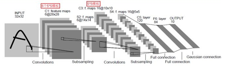
  事实是：每一个卷积核要感受前一层的所有feature_maps

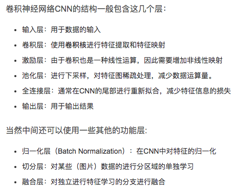
卷积神经网络(Convolutional Neural Network, CNN)是深度学习技术中极具代表的网络结构之一, CNN相较于传统的图像处理算法的优点之一在于，避免了对图像复杂的前期预处理过程（提取人工特征等），可以直接输入原始图像。

图像处理中，往往会将图像看成是一个或多个的二维向量，比如MNIST手写体图片就可以看做是一个28 × 28的二维向量（黑白图片，只有一个颜色通道；如果是RGB表示的彩色图片则有三个颜色通道，可表示为三张二维向量）。传统的神经网络都是采用全连接的方式，即输入层到隐藏层的神经元都是全部连接的，这样做将导致参数量巨大，使得网络训练耗时甚至难以训练，而CNN则通过局部连接、权值共享等方法避免这一困难。

• Why using the patches of images as input instead of the whole images?

  I saw this phenomenon when I read papers about crowd counting with CNN, like S-CNN MCNN. And according to the paper S-CNN, the complete image is divided in 9 non-overlapping patches so that crowd characteristics like density, appearance etc. can be assumed to be consistent in a given patch for a crowd scene.

• What is fine-tune of CNN model? fine tuning

• 如何理解“卷积运算，可以使原信号特征增强，并且降低噪音”？？

• 为什么神经网络可以提取特征？？

• 模型的鲁棒性？？？？

A

1. In machine learning terms, this flashlight is called a filter(or sometimes referred to as a neuron or a kernel) and the region that it is shining over is called the receptive field.

2. A very important note is that the depth of this filter has to be the same as the depth of the input (this makes sure that the math works out), so the dimensions of this filter is 5 x 5 x 3.

   

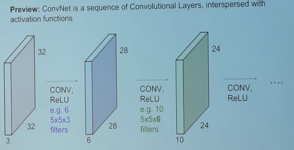
3. For an input image with size $N \times N \times C$, after going through a filter $5 \times 5$, we have an output feature map with size $(N-5+1) \times (N-5+1) \times 1$.

   output_size = (Height-Filter)/stride+1.

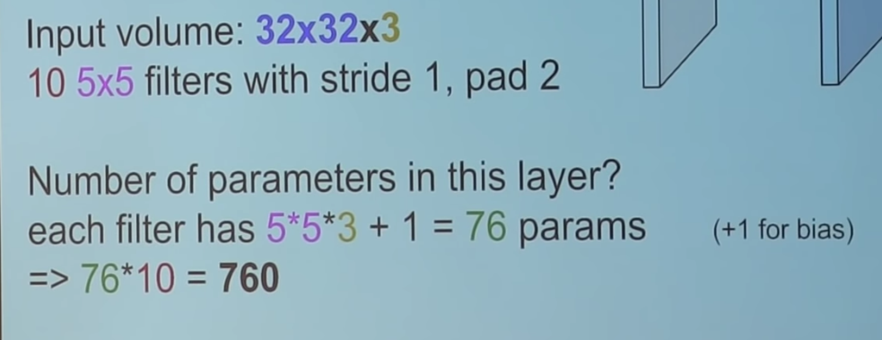
4. weight number

   

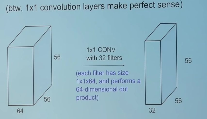
5. $1 \times 1$ filter size

   

6. ​

CNN的引入

直观理解深度学习卷积部分

ThumbsUp

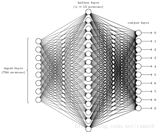
在人工的全连接神经网络中，每相邻两层之间的每个神经元之间都是有边相连的。当输入层的特征维度变得很高时，这时全连接网络需要训练的参数就会增大很多，计算速度就会变得很慢，例如一张黑白的 28×28 的手写数字图片，输入层的神经元就有784个，如下图所示：

CNN层次结构

输入层

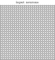
CNN的输入层的输入格式保留了图片本身的结构。

对于黑白的 28×2828×28 的图片，CNN的输入是一个 28×2828×28 的的二维神经元，如下图所示：

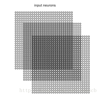
而对于RGB格式的$28\times 28$图片，CNN的输入则是一个$3\times 28\times 28$的三维神经元（RGB中的每一个颜色通道都有一个 $28\times 28$的矩阵）

卷积层

两个重要的概念：

• local receptive fields（局部视野野）
• shared weights（权值共享）

局部感受野

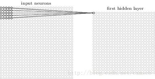
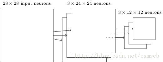
相比传统的每个神经元与前一层的所有神经元全连接，CNN中每个神经元只与前一层的部分神经元连接，俗称局部感受。如下图，假设输入的是一个 $28\times 28$的的二维神经元，我们定义$5\times 5$的 一个 local receptive fields（感受视野），即 隐藏层的神经元与输入层的$5\times 5$个神经元相连，这个5*5的区域就称之为Local Receptive Fields，每一条直线对应一个权重$w$。

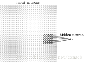
每个神经元只与$5\times5$大小范围的神经元连接，如果步长是1，则两个神经元之间的感受区域有重叠，所以下一层共需要神经元个数是$(28\times 28) \div(5\times5)=(28-(5-1))\times(28-(5-1))=24\times24$

移动的步长为1：从左到右扫描，每次移动 1 格，扫描完之后，再向下移动一格，再次从左到右扫描。

过滤器-卷积核-Filters-权重$w$-(神经元局部感受的模板)

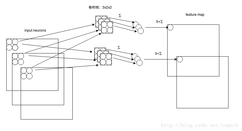
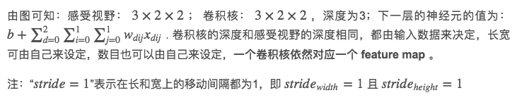
一个感受野带有一个卷积核，将感受野对输入的扫描间隔称为步长(Stride)，当步长比较大时(stride>1)，为了扫描到边缘的一些特征，感受视野可能会“出界”，这时需要对边界扩充(pad)，边界扩充可以设为 00 或 其他值。步长 和 边界扩充值的大小由用户来定义。

比如前一层是$5\times5$, 感受野大小是$2\times2$, 步长2，可以发现最右的边界是无法扫描，所以可以对前一层进行padding，扩充成$6\times6$。

卷积核的权重矩阵的值，便是卷积神经网络的参数，为了有一个偏移项 $b$，卷积核可附带一个偏移项 bb ，它们的初值可以随机来生成，可通过训练进行变化。

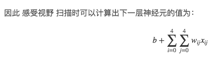
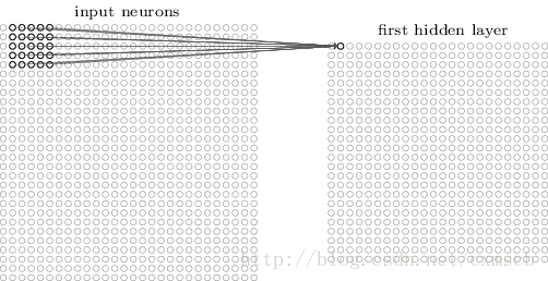
我们将通过 一个带有卷积核的感受视野 扫描生成的下一层神经元矩阵 称为 一个feature map (特征映射图)，如下图的右边便是一个 feature map：

因此在同一个 feature map 上的神经元使用的卷积核是相同的，因此这些神经元 shared weights，共享卷积核中的权值和附带的偏移。一个 feature map 对应 一个卷积核，若我们使用 3 个不同的卷积核，可以输出3个feature map：（感受视野：5×5，布长stride：1）

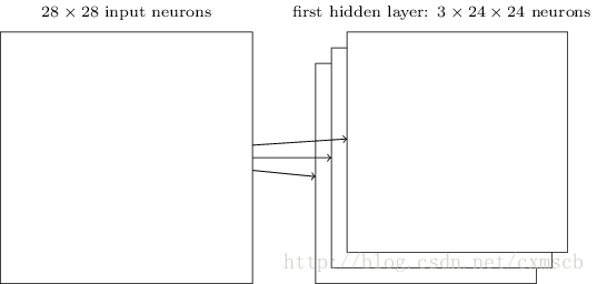
因此在CNN的卷积层，我们需要训练的参数大大地减少到了 (5×5+1)×3=78个。

假设输入的是 $28\times28$的RGB图片，即输入的是一个 $3×28×28$的的二维神经元，这时卷积核的大小不只用长和宽来表示，还有深度，感受视野也对应的有了深度。如下图所示：

RGB图像在CNN中如何进行convolution? - 知乎 https://www.zhihu.com/question/46607672

https://blog.csdn.net/u014114990/article/details/51125776

池化层(下采样)

当输入经过卷积层时，若感受视野比较小，布长stride比较小，得到的feature map （特征图）还是比较大，可以通过池化层来对每一个 feature map 进行降维操作，输出的深度还是不变的，依然为 feature map 的个数。

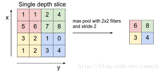
池化层也有一个“池化视野（filter）”来对feature map矩阵进行扫描，对“池化视野”中的矩阵值进行计算，一般有两种计算方式：

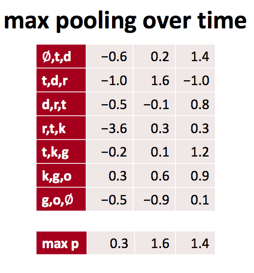
• Max pooling：取“池化视野”矩阵中的最大值
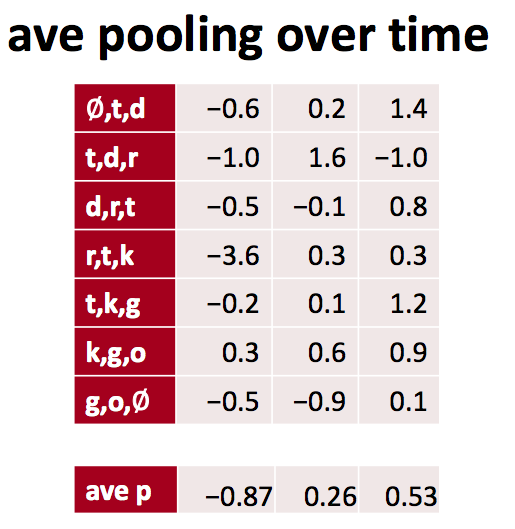
• Average pooling：取“池化视野”矩阵中的平均值

扫描的过程中同样地会涉及的扫描布长stride，扫描方式同卷积层一样，先从左到右扫描，结束则向下移动布长大小，再从左到右。如下图示例所示：

最后可将 3 个 $24\times24$ 的 feature map 下采样得到 3 个 $24\times24$ 的特征矩阵：

全连接层

全连接层主要对特征进行重新拟合，减少特征信息的丢失。用户指定全连接层的神经元个数，然后每个神经元都与前一层的所有神经元连接，计算。

输出层

输出层主要准备做好最后目标结果的输出，用户指定神经元个数，如果是2分类问题，就设置两个神经元，每一个神经元输出某种分类的概率；十分类就10个神经元，属于全连接。

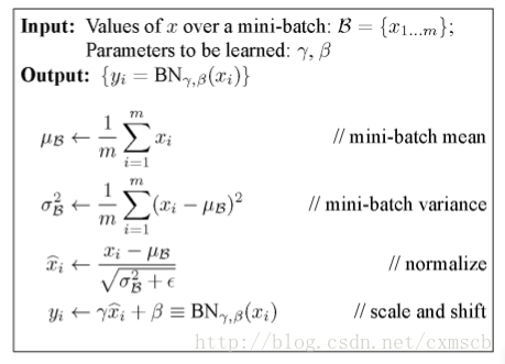
归一化层(Batch Normalization)

实现了在神经网络层的中间进行预处理的操作，即在上一层的输入归一化处理后再进入网络的下一层，这样可有效地防止“梯度弥散”，加速网络训练。在卷积神经网络中进行批量归一化时，一般对 未进行ReLu激活的 feature map进行批量归一化，输出后再作为激励层的输入，可达到调整激励函数偏导的作用。

近邻归一化(Local Response Normalization)

融合层

融合层可以对切分层进行融合，也可以对不同大小的卷积核学习到的特征进行融合。例如在GoogleLeNet 中，使用多种分辨率的卷积核对目标特征进行学习，通过 padding 使得每一个 feature map 的长宽都一致，之后再将多个 feature map 在深度上拼接在一起：

融合的方法有几种，一种是特征矩阵之间的拼接级联，另一种是在特征矩阵进行运算 (+,−,x,max,conv)(+,−,x,max,conv)。

parameters setting

图像归一化

CNN in NLP

Since CNNs, unlike RNNs, can output only fixed sized vectors, the natural fit for them seem to be in the classification tasks such as Sentiment Analysis, Spam Detection or Topic Categorization.

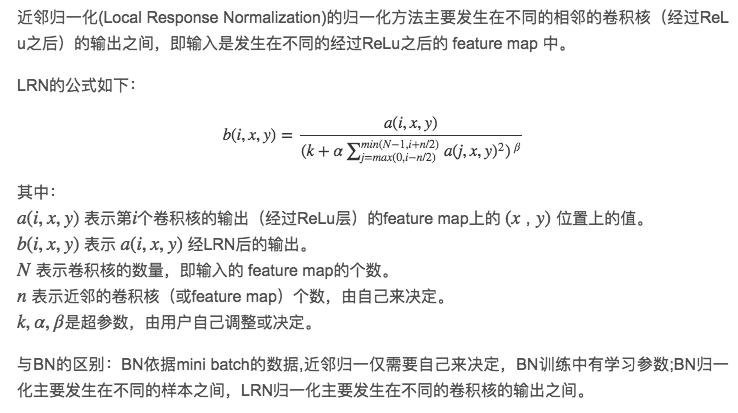
In computer vision tasks, the filters used in CNNs slide over patches of an image whereas in NLP tasks, the filters slide over the sentence matrices, a few words at a time.

Input

Instead of image pixels, the input to most NLP tasks are sentences or documents represented as a matrix. Each row of the matrix corresponds to one token, typically a word, but it could be a character. That is, each row is vector that represents a word. Typically, these vectors are word embeddings (low-dimensional representations) like word2vec or GloVe, but they could also be one-hot vectors that index the word into a vocabulary. For a 10 word sentence using a 100-dimensional embedding we would have a 10×100 matrix as our input. That’s our “image”.

Fliter

In vision, our filters slide over local patches of an image, but in NLP we typically use filters that slide over full rows of the matrix (words). Thus, the “width” of our filters is usually the same as the width of the input matrix. The height, or region size, may vary, but sliding windows over 2-5 words at a time is typical.

Padding

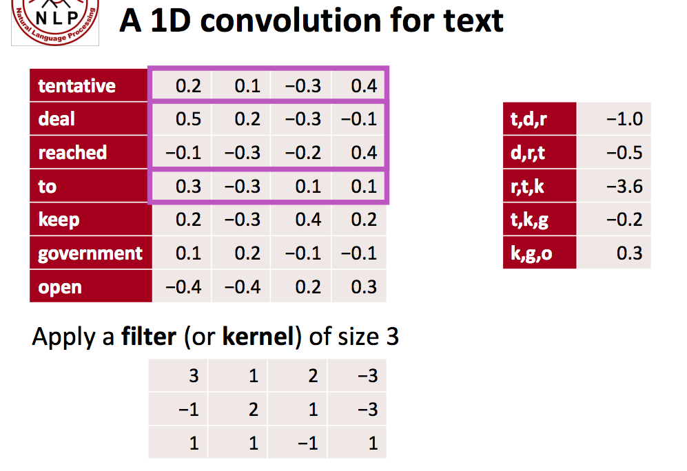
We also have zero-padding in nlp, where all elements that would fall outside of the matrix are taken to be zero. By doing this you can apply the filter to every element of your input matrix, and get a larger or equally sized output. Adding zero-padding is also called wide convolution**, and not using (zero-)padding would be a *narrow convolution*.

Channel

The last concept we need to understand are channels. Channels are different “views” of your input data. For example, in image recognition you typically have RGB (red, green, blue) channels. You can apply convolutions across channels, either with different or equal weights. In NLP you could imagine having various channels as well: You could have a separate channels for different word embeddings (word2vec and GloVe for example), or you could have a channel for the same sentence represented in different languages, or phrased in different ways.

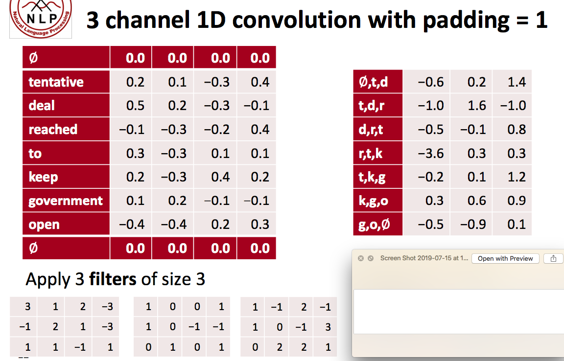
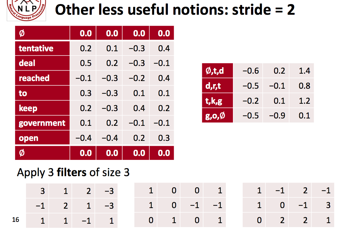
Stride Size

Pooling

Why pooling? There are a couple of reasons. One property of pooling is that it provides a fixed size output matrix, which typically is required for classification. For example, if you have 1,000 filters and you apply max pooling to each, you will get a 1000-dimensional output, regardless of the size of your filters, or the size of your input. This allows you to use variable size sentences, and variable size filters, but always get the same output dimensions to feed into a classifier.

Pooling also reduces the output dimensionality but (hopefully) keeps the most salient information. You can think of each filter as detecting a specific feature, such as detecting if the sentence contains a negation like “not amazing” for example. If this phrase occurs somewhere in the sentence, the result of applying the filter to that region will yield a large value, but a small value in other regions. By performing the max operation you are keeping information about whether or not the feature appeared in the sentence, but you are losing information about where exactly it appeared. But isn’t this information about locality really useful? Yes, it is and it’s a bit similar to what a bag of n-grams model is doing. You are losing global information about locality (where in a sentence something happens), but you are keeping local information captured by your filters, like “not amazing” being very different from “amazing not”.

In imagine recognition, pooling also provides basic invariance to translating (shifting) and rotation. When you are pooling over a region, the output will stay approximately the same even if you shift/rotate the image by a few pixels, because the max operations will pick out the same value regardless.

Architecture

link

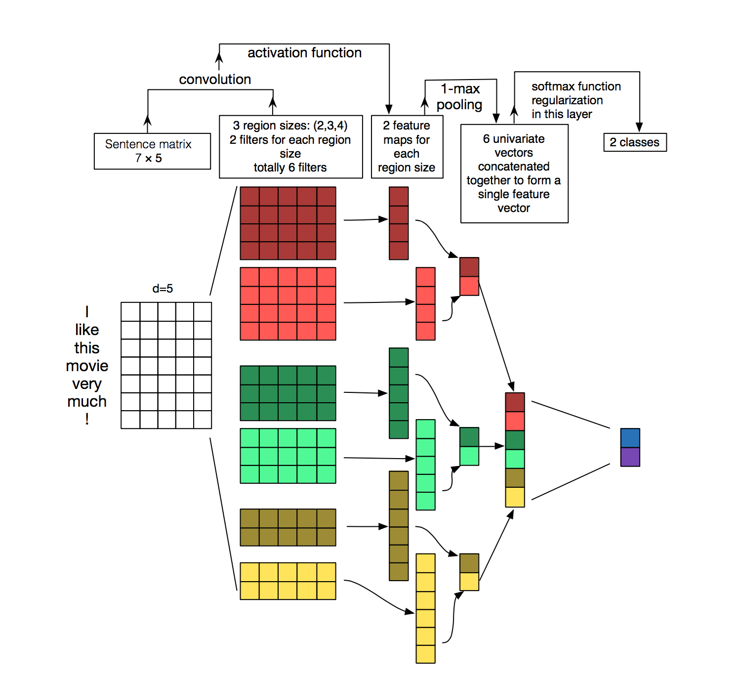
llustration of a Convolutional Neural Network (CNN) architecture for sentence classification. Here we depict three filter region sizes: 2, 3 and 4, each of which has 2 filters. Every filter performs convolution on the sentence matrix and generates (variable-length) feature maps. Then 1-max pooling is performed over each map, i.e., the largest number from each feature map is recorded. Thus a univariate feature vector is generated from all six maps, and these 6 features are concatenated to form a feature vector for the penultimate layer. The final softmax layer then receives this feature vector as input and uses it to classify the sentence; here we assume binary classification and hence depict two possible output states. Source: Zhang, Y., & Wallace, B. (2015). A Sensitivity Analysis of (and Practitioners’ Guide to) Convolutional Neural Networks for Sentence Classification.

Input

The example is “I like this movie very much!”, there are 6 words here and the exclamation mark is treated like a word – some researchers do this differently and disregard the exclamation mark – in total there are 7 words in the sentence. The authors chose 5 to be the dimension of the word vectors. We let s denote the length of sentence and d denote the dimension of the word vector, hence we now have a sentence matrix of the shape s x d, or 7 x 5.

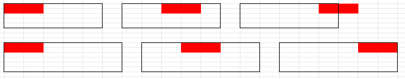
Filters

One of the desirable properties of CNN is that it preserves 2D spatial orientation in computer vision. Texts, like pictures, have an orientation. Instead of 2-dimensional, texts have a one-dimensional structure where words sequence matter. We also recall that all words in the example are each replaced by a 5-dimensional word vector, hence we fix one dimension of the filter to match the word vectors (5) and vary the region size, h. Region size refers to the number of rows – representing word – of the sentence matrix that would be filtered.

In the figure, #filters are the illustrations of the filters, not what has been filtered out from the sentence matrix by the filter, the next paragraph would make this distinction clearer. Here, the authors chose to use 6 filters – 2 complementary filters to consider (2,3,4) words.

Featuremaps

For filters with size being 4, the output featuremap size should be (7-4)/1+1=4. Similarly, we have output featuremaps of 5 and 6 respectively for filter size 3 and 2.

Maxpooling

For each featuremap, we perform 1-max pooling and extract the largest number.

Softmax

After 1-max pooling, we are certain to have a fixed-length vector of 6 elements ( = number of filters = number of filters per region size (2) x number of region size considered (3)). This fixed length vector can then be fed into a softmax (fully-connected) layer to perform the classification. The error from the classification is then back-propagated back into the following parameters as part of learning:

• The w matrices that produced o
• The bias term that is added to o to produce c
• Word vectors (optional, use validation performance to decide)

CNN Applications in NLP

The most natural fit for CNNs seem to be classifications tasks, such as Sentiment Analysis, Spam Detection or Topic Categorization. Convolutions and pooling operations lose information about the local order of words, so that sequence tagging as in PoS Tagging or Entity Extraction is a bit harder to fit into a pure CNN architecture (though not impossible, you can add positional features to the input).

Pytorch Implementation

link

import torch
import torch.optim as optim
import torch.nn as nn
import torch.nn.functional as F
import torch
from torchtext import data
from torchtext import datasets
import random
import spacy

# https://github.com/bentrevett/pytorch-sentiment-analysis/blob/master/4%20-%20Convolutional%20Sentiment%20Analysis.ipynb

SEED = 1234

torch.manual_seed(SEED)
torch.backends.cudnn.deterministic = True

spacy_en = spacy.load('en')
def tokenizer(text): # create a tokenizer function
    return [tok.text for tok in spacy_en.tokenizer(text)]

TEXT = data.Field(tokenize = tokenizer)
LABEL = data.LabelField(dtype = torch.float)

train_data, test_data = datasets.IMDB.splits(TEXT, LABEL)

train_data, valid_data = train_data.split(random_state = random.seed(SEED))

MAX_VOCAB_SIZE = 25_000

TEXT.build_vocab(train_data,
                 max_size = MAX_VOCAB_SIZE,
                 vectors = "glove.6B.100d",
                 unk_init = torch.Tensor.normal_)

LABEL.build_vocab(train_data)
BATCH_SIZE = 64

device = torch.device('cuda' if torch.cuda.is_available() else 'cpu')

train_iterator, valid_iterator, test_iterator = data.BucketIterator.splits(
    (train_data, valid_data, test_data),
    batch_size = BATCH_SIZE,
    device = device)

def count_parameters(model):
    return sum(p.numel() for p in model.parameters() if p.requires_grad)

def binary_accuracy(preds, y):
    """
    Returns accuracy per batch, i.e. if you get 8/10 right, this returns 0.8, NOT 8
    """
    #round predictions to the closest integer
    rounded_preds = torch.round(torch.sigmoid(preds))
    correct = (rounded_preds == y).float() #convert into float for division
    acc = correct.sum() / len(correct)
    return acc

def train(model, iterator, optimizer, criterion):
    epoch_loss = 0
    epoch_acc = 0
    model.train()

    for batch in iterator:
        optimizer.zero_grad()

        batch_ = batch.text #torch.Size([1225, 64])

        predictions = model(batch_).squeeze(1)

        loss = criterion(predictions, batch.label)

        acc = binary_accuracy(predictions, batch.label)

        loss.backward()

        optimizer.step()

        epoch_loss += loss.item()
        epoch_acc += acc.item()

    return epoch_loss / len(iterator), epoch_acc / len(iterator)

class TextCNN(nn.Module):
    def __init__(self,vocab_size, embedding_dim, n_filters, filter_sizes, output_dim, dropout, pad_idx):
        super(TextCNN,self).__init__()
        self.embedding = nn.Embedding(vocab_size,embedding_dim,pad_idx)
        self.conv1 = nn.Conv2d(in_channels=1,out_channels=n_filters,kernel_size=(filter_sizes[0],embedding_dim))
        self.conv2 = nn.Conv2d(in_channels=1,out_channels=n_filters,kernel_size=(filter_sizes[1],embedding_dim))
        self.conv3 = nn.Conv2d(in_channels=1,out_channels=n_filters,kernel_size=(filter_sizes[2],embedding_dim))
        self.fc = nn.Linear(n_filters*len(filter_sizes),output_dim)
        self.dropout = nn.Dropout(p=dropout)

    def forward(self, text):
        #text.shape = (sent_length,batch_size), sent_length is varing
        text = torch.transpose(text, 0, 1) #(batch_size,sent_length)=(64,1225)
        text_embedding = self.embedding(text) # shape = (batch_size,sent_length,embedding_size)=(64,1225,100)
        
        # since we use conv2d, the input should be (batch,channel,height,width)
        text_embedding = torch.unsqueeze(text_embedding,dim=1)
        
        #kernel_size is (?,embedding_dim), so output is (batch,filter_num,??,1)
        conv1 = F.relu(self.conv1(text_embedding)) #Size([64, 100, 1223, 1])
        conv2 = F.relu(self.conv2(text_embedding)) #Size([64, 100, 1222, 1])
        conv3 = F.relu(self.conv3(text_embedding)) #Size([64, 100, 1221, 1])

        pooling1 = F.max_pool1d(conv1.squeeze(),conv1.size(2))
        pooling2 = F.max_pool1d(conv2.squeeze(),conv2.size(2))
        pooling3 = F.max_pool1d(conv3.squeeze(),conv3.size(2))

        cat = torch.cat((pooling1,pooling2,pooling3),dim=1).squeeze() #Size([64,300,1,1]->[64,300])
        dropout = self.dropout(cat)
        output = self.fc(dropout) #fully-connected layers can only be (batch_size,dim)
        return output

if __name__ == '__main__':
    INPUT_DIM = len(TEXT.vocab) #25002
    EMBEDDING_DIM = 100
    N_FILTERS = 100
    FILTER_SIZES = [3, 4, 5]
    OUTPUT_DIM = 1
    DROPOUT = 0.5
    PAD_IDX = TEXT.vocab.stoi[TEXT.pad_token]
    model = TextCNN(INPUT_DIM, EMBEDDING_DIM, N_FILTERS, FILTER_SIZES, OUTPUT_DIM, DROPOUT, PAD_IDX)
    print(f'The model has {count_parameters(model):,} trainable parameters')
    pretrained_embeddings = TEXT.vocab.vectors
    model.embedding.weight.data.copy_(pretrained_embeddings)
    UNK_IDX = TEXT.vocab.stoi[TEXT.unk_token]
    model.embedding.weight.data[UNK_IDX] = torch.zeros(EMBEDDING_DIM)
    model.embedding.weight.data[PAD_IDX] = torch.zeros(EMBEDDING_DIM)
    optimizer = optim.Adam(model.parameters())
    criterion = nn.BCEWithLogitsLoss()
    model = model.to(device)
    criterion = criterion.to(device)
    N_EPOCHS = 5
    best_valid_loss = float('inf')
    for epoch in range(N_EPOCHS):
        train_loss, train_acc = train(model, train_iterator, optimizer, criterion)
        print(f'\tTrain Loss: {train_loss:.3f} | Train Acc: {train_acc*100:.2f}%')

Tensorflow代码

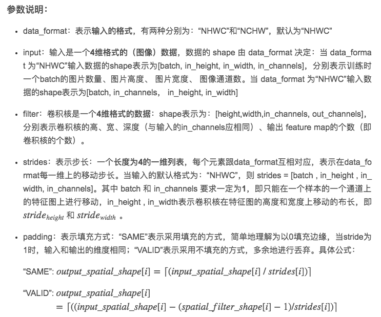
卷积层tf.nn.conv2d()

tf.nn.conv2d(input, filter, strides, padding, use_cudnn_on_gpu=None, data_format=None, name=None)

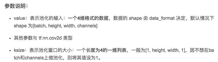
池化层tf.nn.max_pool()

tf.nn.max_pool( value, ksize,strides,padding,data_format=’NHWC’,name=None) 
#或者 
tf.nn.avg_pool(…)

归一化层tf.nn.batch_normalization()

batch_normalization( x,mean,variance,offset,scale, variance_epsilon,name=None)

• mean 和 variance 通过 tf.nn.moments 来进行计算：
  batch_mean, batch_var = tf.nn.moments(x, axes = [0, 1, 2], keep_dims=True)，注意axes的输入。对于以feature map 为维度的全局归一化，若feature map 的shape 为[batch, height, width, depth]，则将axes赋值为[0, 1, 2]
• x 为输入的feature map 四维数据，offset、scale为一维Tensor数据，shape 等于 feature map 的深度depth。

代码示例

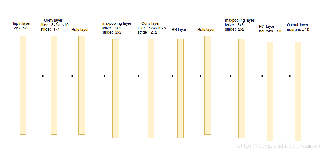
通过搭建卷积神经网络来实现sklearn库中的手写数字识别，搭建的卷积神经网络结构如下图所示：

import tensorflow as tf
from sklearn.datasets import load_digits
import numpy as np

digits = load_digits()
x_data = digits.data.astype(np.float32)
y_data = digits.target.astype(np.float32)
print(y_data) # [0. 1. 2. ... 8. 9. 8.]
y_data = y_data.reshape(-1,1)
print(y_data)
# [[0.]
#  [1.]
#  [2.]
#  ...
#  [8.]
#  [9.]
#  [8.]]
print(x_data.shape) #(1797,64)

from sklearn.preprocessing import MinMaxScaler # 将属性缩放到一个指定的最大和最小值（通常是1-0）之间
scaler = MinMaxScaler()
x_data = scaler.fit_transform(x_data)
from sklearn.preprocessing import OneHotEncoder
y = OneHotEncoder().fit_transform(y_data).todense()
print(y)
# [[1. 0. 0. ... 0. 0. 0.]
#  [0. 1. 0. ... 0. 0. 0.]
#  [0. 0. 1. ... 0. 0. 0.]
#  ...
#  [0. 0. 0. ... 0. 1. 0.]
#  [0. 0. 0. ... 0. 0. 1.]
#  [0. 0. 0. ... 0. 1. 0.]]

#转换为图片的格式 （batch，height，width，channels）
x = x_data.reshape(-1,8,8,1) #-1表示适应大小，原来是64长度，变成8*8，则适应大小是1，即one batch的图片数目是1
batch_size = 8 # 使用MBGD算法，设定batch_size为8
def generatebatch(x,y,n_examples,batch_size):
    for batch_i in range(n_examples // batch_size):
        start = batch_i * batch_size
        end = start + batch_size
        batch_xs = x[start:end]
        batch_ys = y[start:end]
        yield batch_xs, batch_ys  # 生成每一个batch

#输入层
tf.reset_default_graph()
tf_x = tf.placeholder(tf.float32,[None,8,8,1]) #灰度图片，CHANEL是1
tf_y = tf.placeholder(tf.float32,[None,10])
#卷积层+激活层
conv_filter_w1 = tf.Variable(tf.random_normal([3,3,1,10])) #shape:10个filter，size是3*3，灰度图片1
conv_filter_b1 = tf.Variable(tf.random_normal([10])) #10个filter
relu_feature_maps1 = tf.nn.relu(
    tf.nn.conv2d(tf.x,conv_filter_w1,
                 strides=[1,1,1,1],#batch和in_chanel是1，1*1是移动步
                 padding='same')
    +conv_filter_b1)
#池化层
max_pool1 = tf.nn.max_pool(relu_feature_maps1,
                           ksize=[1,3,3,1],
                           strides=[1,2,2,1],
                           padding='same')

#卷积层
conv_filter_w2 = tf.Variable(tf.random_normal([3,3,10,5])) #10是in_chanel,与输入的in_chanel相同，5是feature_maps数目
conv_filter_b2 = tf.Variable(tf.random_normal([5])) #与神经元个数相同
conv_out2 = tf.nn.conv2d(relu_feature_maps1,conv_filter_w2,strides=[1,2,2,1],padding='SAME')+conv_filter_b2

#BN归一化层+激励层
batch_mean, batch_var = tf.nn.moments(conv_out2, [0, 1, 2], keep_dims=True)
shift = tf.Variable(tf.zeros([5]))
scale = tf.Variable(tf.ones([5]))
epsilon = 1e-3
BN_out = tf.nn.batch_normalization(conv_out2, batch_mean, batch_var, shift, scale, epsilon)
relu_BN_maps2 = tf.nn.relu(BN_out)

#池化层
max_pool2 = tf.nn.max_pool(BN_out,ksize=[1,3,3,1],strides=[1,2,2,1],padding='SAME')

#特征图展开，输入大小是8*8，两次pooling，变成2*2，而且有5个神经元，则展开大小是2*2*5
max_pool2_flat = tf.reshape(max_pool2,[-1,2*2*5])
#全连接层
fc_w1 = tf.Variable(tf.random_normal([2*2*5,50])) #50神经元
fc_b1 = tf.Variable(tf.random_normal([50]))
fc_out1 = tf.nn.relu(tf.matmul(max_pool2_flat,fc_w1)+fc_b1)
#输出层
out_w1 = tf.Variable(tf.random_normal([50,10]))
out_b1 = tf.Variable(tf.random_normal([10]))
pred = tf.nn.softmax(tf.matmul(fc_out1,out_w1)+out_b1)

loss = -tf.reduce_mean(tf_y*tf.log(tf.clip_by_value(pred,1e-11,1.0)))
train_step = tf.train.AdamOptimizer(1e-3).minimize(loss)
y_pred = tf.arg_max(pred,1)
bool_pred = tf.equal(tf.arg_max(tf_y,1),y_pred)
accuracy = tf.reduce_mean(tf.cast(bool_pred,tf.float32)) # 准确率
with tf.Session() as sess:
    sess.run(tf.global_variables_initializer())
    for epoch in range(1000): # 迭代1000个周期
        for batch_xs,batch_ys in generatebatch(x,y,y.shape[0],batch_size): # 每个周期进行MBGD算法
            sess.run(train_step,feed_dict={tf_x:batch_xs , tf_y:batch_ys})
        if(epoch%100==0):
            res = sess.run(accuracy,feed_dict={tf_x:x,tf_y:y})
            print (epoch,res)
    res_ypred = y_pred.eval(feed_dict={tf_x:x,tf_y:y}).flatten() # 只能预测一批样本，不能预测一个样本
    print (res_ypred)

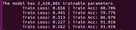
在第100次个batch size 迭代时，准确率就快速接近收敛了，这得归功于Batch Normalization 的作用！需要注意的是，这个模型还不能用来预测单个样本，因为在进行BN层计算时，单个样本的均值和方差都为0，会得到相反的预测效果，解决方法详见归一化层。

from sklearn.metrics import  accuracy_score
print(accuracy_score(Y_data,res_ypred.reshape(-1,1)))
# 0.998887033945

CNN结构扩展

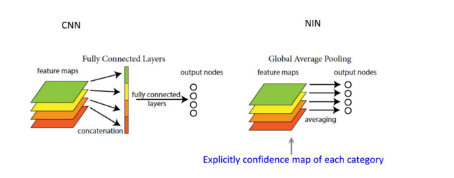
GAP(Global Average Pooling)

[Ref1] [Ref2]

GAP是用来代替全连接层，由于全连接层过多的参数重要到会造成过拟合，所以GAP放弃了对前一层的全连接，使用pooling来降低参数。global average pooling 与 average pooling 的差别就在 “global” 这一个字眼上。global 与 local 在字面上都是用来形容 pooling 窗口区域的。 local 是取 feature map 的一个子区域求平均值，然后滑动这个子区域； global 显然就是对整个 feature map 求平均值了。因此，global average pooling 的最后输出结果仍然是 10 个 feature map，而不是一个，只不过每个 feature map 只剩下一个像素罢了。这个像素就是求得的平均值。

举个例子

假如，最后的一层的数据是10个66的特征图，global average pooling是将每一张特征图计算所有像素点的均值，输出一个数据值，这样10 个特征图就会输出10个数据点，将这些数据点组成一个110的向量的话，就成为一个特征向量，就可以送入到softmax的分类中计算了

Reference

Building a convolutional neural network for natural language processing