Keras

Keras使用技巧。

TODO

• [ ] LSTM
• [ ] CONV1D
• [ ] TIMEDISTRIBUTED-VIDEOS
• [ ] FIT_GENERATOR
• [ ] STATEFUL_RNN

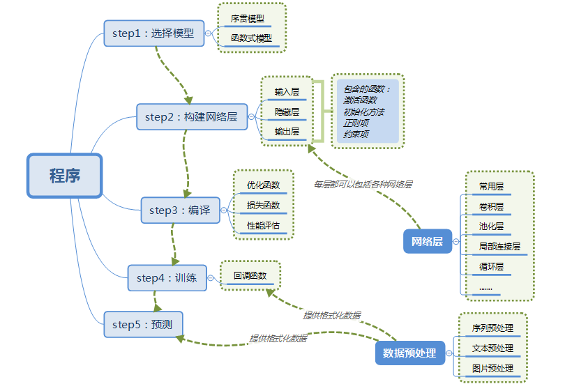
Keras模块结构

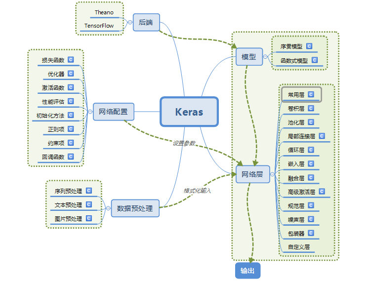
Keras构建神经网络

Models

There are two ways to implement a keras model, Sequential and Model. We will use an image classification example to see how these ways work and their corresponding properties.

We use MNIST hand-written recognition as the example. We will implement a three-layers convolution network, i.e., input_layer -> conv2d -> conv2d -> dense -> output_layer

from keras.models import Sequential
from keras.layers import Dense, Conv2D, Flatten
from keras.datasets import mnist
from keras.utils import to_categorical
(X_train, y_train), (X_test, y_test) = mnist.load_data()
X_train = X_train.reshape(60000,28,28,1)
X_test = X_test.reshape(10000,28,28,1)
y_train = to_categorical(y_train)
y_test = to_categorical(y_test)
model = Sequential()
#add model layers
model.add(Conv2D(64, kernel_size=3, activation='relu', input_shape=(28,28,1),name='conv1'))
model.add(Conv2D(32, kernel_size=3, activation='relu',name='conv2'))
model.add(Flatten(name='flatten'))
model.add(Dense(10, activation='softmax',name='dense'))
model.compile(optimizer='adam', loss='categorical_crossentropy', metrics=['accuracy'])

Attributes

model.layers: return a flattened list of the layers comprising the model.

print(model.layers)
##[<keras.layers.convolutional.Conv2D object at 0x11b62a780>, <keras.layers.convolutional.Conv2D object at 0x11b63df98>, <keras.layers.core.Flatten object at 0x11eb17588>, <keras.layers.core.Dense object at 0x11eb170f0>]

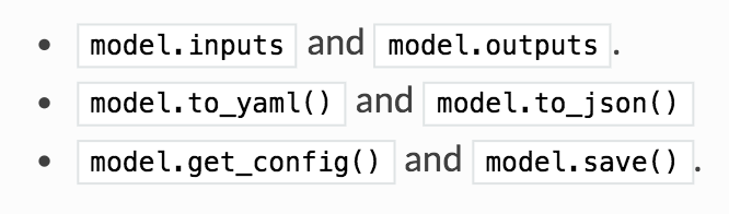
model.inputs: return the list of input tensors of the model.

print(model.inputs)
##[<tf.Tensor 'conv1_input:0' shape=(?, 28, 28, 1) dtype=float32>]

model.outputs: return the list of output tensors of the model.

print(model.outputs)
##[<tf.Tensor 'dense/Softmax:0' shape=(?, 10) dtype=float32>]

model.summary: prints a summary representation of the model.

_________________________________________________________________
Layer (type)                 Output Shape              Param #   
=================================================================
conv1 (Conv2D)               (None, 26, 26, 64)        640       
_________________________________________________________________
conv2 (Conv2D)               (None, 24, 24, 32)        18464     
_________________________________________________________________
flatten (Flatten)            (None, 18432)             0         
_________________________________________________________________
dense (Dense)                (None, 10)                184330    
=================================================================
Total params: 203,434
Trainable params: 203,434
Non-trainable params: 0
_________________________________________________________________

model.get_weights(): return a list of all weights tensors as Numpy arrays, where weights are stored in model.get_weights()[0] and bias are stored in model.get_weights()[2].

print(model.get_weights())

Model subclassing

In addition to these two types of models, you may create your own fully-customizable models by subclassing the Model class and implementing your own forward pass in the call method.

import keras

class SimpleMLP(keras.Model):

    def __init__(self, use_bn=False, use_dp=False, num_classes=10):
        super(SimpleMLP, self).__init__(name='mlp')
        self.use_bn = use_bn
        self.use_dp = use_dp
        self.num_classes = num_classes

        self.dense1 = keras.layers.Dense(32, activation='relu')
        self.dense2 = keras.layers.Dense(num_classes, activation='softmax')
        if self.use_dp:
            self.dp = keras.layers.Dropout(0.5)
        if self.use_bn:
            self.bn = keras.layers.BatchNormalization(axis=-1)

    def call(self, inputs):
        x = self.dense1(inputs)
        if self.use_dp:
            x = self.dp(x)
        if self.use_bn:
            x = self.bn(x)
        return self.dense2(x)

model = SimpleMLP()
model.compile(...)
model.fit(...)

In call, you may specify custom losses by calling self.add_loss(loss_tensor) (like you would in a custom layer).

But in subclassed models, the following methods and attributes are not available:

Model class API

Methods

compile

compile(optimizer, loss=None, metrics=None, loss_weights=None, sample_weight_mode=None, weighted_metrics=None, target_tensors=None)

fit

fit(x=None, y=None, batch_size=None, epochs=1, verbose=1, callbacks=None, validation_split=0.0, validation_data=None, shuffle=True, class_weight=None, sample_weight=None, initial_epoch=0, steps_per_epoch=None, validation_steps=None, validation_freq=1)

• verbose: Integer. 0, 1, or 2. Verbosity mode. 0 = silent, 1 = progress bar, 2 = one line per epoch.
• A History object. Its History.history attribute is a record of training loss values and metrics values at successive epochs, as well as validation loss values and validation metrics values (if applicable).

evaluate

evaluate(x=None, y=None, batch_size=None, verbose=1, sample_weight=None, steps=None, callbacks=None)

Returns scalar test loss (if the model has a single output and no metrics) or list of scalars (if the model has multiple outputs and/or metrics). The attribute model.metrics_names will give you the display labels for the scalar outputs.

Computation is done in batches.

• verbose: 0 or 1. Verbosity mode. 0 = silent, 1 = progress bar.

predict

predict(x, batch_size=None, verbose=0, steps=None, callbacks=None)

• verbose: Verbosity mode, 0 or 1.

train_on_batch

train_on_batch(x, y, sample_weight=None, class_weight=None)

• Scalar training loss (if the model has a single output and no metrics) or list of scalars (if the model has multiple outputs and/or metrics). The attribute model.metrics_names will give you the display labels for the scalar outputs.
• Runs a single gradient update on a single batch of data.

test_on_batch

test_on_batch(x, y, sample_weight=None)

• Test the model on a single batch of samples.
• Scalar test loss (if the model has a single output and no metrics) or list of scalars (if the model has multiple outputs and/or metrics). The attribute model.metrics_names will give you the display labels for the scalar outputs.

predict_on_batch

predict_on_batch(x)

fit_generator

fit_generator(generator, steps_per_epoch=None, epochs=1, verbose=1, callbacks=None, validation_data=None, validation_steps=None, validation_freq=1, class_weight=None, max_queue_size=10, workers=1, use_multiprocessing=False, shuffle=True, initial_epoch=0)

• Return a History object. Its History.history attribute is a record of training loss values and metrics values at successive epochs, as well as validation loss values and validation metrics values (if applicable).

• generator: A generator or an instance of Sequence (keras.utils.Sequence) object in order to avoid duplicate data when using multiprocessing. The output of the generator must be either

  • a tuple (inputs, targets)
  • a tuple (inputs, targets, sample_weights).

  This tuple (a single output of the generator) makes a single batch. Therefore, all arrays in this tuple must have the same length (equal to the size of this batch). Different batches may have different sizes. For example, the last batch of the epoch is commonly smaller than the others, if the size of the dataset is not divisible by the batch size. The generator is expected to loop over its data indefinitely. An epoch finishes when steps_per_epoch batches have been seen by the model.

def generate_arrays_from_file(path):
    while True:
        with open(path) as f:
            for line in f:
                # create numpy arrays of input data
                # and labels, from each line in the file
                x1, x2, y = process_line(line)
                yield ({'input_1': x1, 'input_2': x2}, {'output': y})

model.fit_generator(generate_arrays_from_file('/my_file.txt'),
                    steps_per_epoch=10000, epochs=10)

evaluate_generator

evaluate_generator(generator, steps=None, callbacks=None, max_queue_size=10, workers=1, use_multiprocessing=False, verbose=0)

Evaluates the model on a data generator.

Scalar test loss (if the model has a single output and no metrics) or list of scalars (if the model has multiple outputs and/or metrics). The attribute model.metrics_names will give you the display labels for the scalar outputs.

predict_generator

predict_generator(generator, steps=None, callbacks=None, max_queue_size=10, workers=1, use_multiprocessing=False, verbose=0)

get_layer

get_layer(name=None, index=None)

Retrieves a layer based on either its name (unique) or index.

If name and index are both provided, index will take precedence.

Indices are based on order of horizontal graph traversal (bottom-up).

Return a layer instance.

Layers

Properties

Get weights

layer.get_weights()
layer.set_weights(weights)
layer.get_config():returns a dictionary containing the configuration of the layer.

Get input/output/shape

Whenever you are calling a layer on some input, you are creating a new tensor (the output of the layer), and you are adding a “node” to the layer, linking the input tensor to the output tensor. When you are calling the same layer multiple times, that layer owns multiple nodes indexed as 0, 1, 2…

In previous versions of Keras, you could obtain the output tensor of a layer instance via layer.get_output(), or its output shape via layer.output_shape. You still can (except get_output() has been replaced by the property output). But what if a layer is connected to multiple inputs?

As long as a layer is only connected to one input, there is no confusion, and .output will return the one output of the layer:

a = Input(shape=(280, 256))
lstm = LSTM(32)
encoded_a = lstm(a)
assert lstm.output == encoded_a

If we have multiple inputs:

a = Input(shape=(280, 256))
b = Input(shape=(280, 256))
lstm = LSTM(32)
encoded_a = lstm(a)
encoded_b = lstm(b)
assert lstm.get_output_at(0) == encoded_a
assert lstm.get_output_at(1) == encoded_b

The same is true for the properties input_shape and output_shape: as long as the layer has only one node, or as long as all nodes have the same input/output shape, then the notion of “layer output/input shape” is well defined, and that one shape will be returned by layer.output_shape/layer.input_shape. But if, for instance, you apply the same Conv2D layer to an input of shape (32, 32, 3), and then to an input of shape (64, 64, 3), the layer will have multiple input/output shapes, and you will have to fetch them by specifying the index of the node they belong to:

a = Input(shape=(32, 32, 3))
b = Input(shape=(64, 64, 3))
conv = Conv2D(16, (3, 3), padding='same')
conved_a = conv(a)
# Only one input so far, the following will work:
assert conv.input_shape == (None, 32, 32, 3)
conved_b = conv(b)
# now the `.input_shape` property wouldn't work, but this does:
assert conv.get_input_shape_at(0) == (None, 32, 32, 3)
assert conv.get_input_shape_at(1) == (None, 64, 64, 3)

Obtain output of an intermediate layer

There are two ways to do it. The first one is to create a new model that outputs the layers we want.

from keras.models import Model
complete_model = Model() #create the original model
layer_name = 'my_layer'
intermediate_layer_model = Model(inputs=complete_model.input,outputs=model.get_layer(layer_name).output)
intermediate_output = intermediate_layer_model.predict(data)

Alternatively, we can build a Keras function that will return the output of a certain layer given a certain input, for example:

from keras import backend as K
# with a Sequential model
get_3rd_layer_output = K.function([model.layers[0].input],
                                  [model.layers[3].output])
layer_output = get_3rd_layer_output([x])[0]

Core Layers

Dense()

keras.layers.Dense(units, activation=None, use_bias=True, kernel_initializer='glorot_uniform', bias_initializer='zeros', kernel_regularizer=None, bias_regularizer=None, activity_regularizer=None, kernel_constraint=None, bias_constraint=None)

• It implements the fully-connected multiplication operation: output=activation(dot(input,kernel)+bias), where activation is the element-wise activation function passed as the activation argument, kernelis a weights matrix and bias is a bias vector.
• The input’s shape should be like (batch_size,dim), otherwise, use Flatten() layer to reshape the input.
• The output shape is (batch_size,units)

Flatten()

keras.layers.Flatten()

• Flattens the input. Does not affect the batch size.

Input()

Input(shape=())

• It is used to instantiate a Keras tensor.
• shape: A shape tuple (integer), not including the batch size. For instance, shape=(32,) indicates that the expected input will be batches of 32-dimensional vectors.

Reshape()

keras.layers.Reshape(target_shape)

• target_shape: target shape. Tuple of integers. Does not include the batch axis. Support shape inference using -1 as dimension.
• The shape of output is like (batch_size,)+target_shape

Permute()

keras.layers.Permute(dims)

• Permutes the dimensions of the input according to a given pattern.

RepeatVector()

keras.layers.RepeatVector(n)

• Repeats the input n times. Input: 2D tensor of shape (num_samples, features). output shape: 3D tensor of shape (num_samples, n, features).

Conv2D()

keras.layers.Conv2D(filters, kernel_size, strides=(1, 1), padding='valid', data_format=None, dilation_rate=(1, 1), activation=None, use_bias=True, kernel_initializer='glorot_uniform', bias_initializer='zeros', kernel_regularizer=None, bias_regularizer=None, activity_regularizer=None, kernel_constraint=None, bias_constraint=None)

• 2D convolution layer (e.g. spatial convolution over images).
• This layer creates a convolution kernel that is convolved with the layer input to produce a tensor of outputs.

Conv2DTranspose()

keras.layers.Conv2DTranspose(filters, kernel_size, strides=(1, 1), padding='valid', output_padding=None, data_format=None, dilation_rate=(1, 1), activation=None, use_bias=True, kernel_initializer='glorot_uniform', bias_initializer='zeros', kernel_regularizer=None, bias_regularizer=None, activity_regularizer=None, kernel_constraint=None, bias_constraint=None)

• Transposed convolution layer (sometimes called Deconvolution).

UpSampling2D()

keras.layers.UpSampling2D(size=(2, 2), data_format=None, interpolation='nearest')

• Repeats the rows and columns of the data by size[0] and size[1] respectively.
• input shape (batch_size,rows,cols,channels),

ZeroPadding2D()

keras.layers.ZeroPadding2D(padding=(1, 1), data_format=None)

• This layer can add rows and columns of zeros at the top, bottom, left and right side of an image tensor.

MaxPooling2D()

keras.layers.MaxPooling2D(pool_size=(2, 2), strides=None, padding='valid', data_format=None)

• If None, it will default to pool_size.
• input shape (batch_size, rows, cols, channels), output shape (batch_size, pooled_rows, pooled_cols, channels)

AveragePooling2D()

keras.layers.AveragePooling2D(pool_size=(2, 2), strides=None, padding='valid', data_format=None)

• input shape (batch_size, rows, cols, channels), output shape (batch_size, pooled_rows, pooled_cols, channels)

GlobalMaxPooling2D()

keras.layers.GlobalMaxPooling2D(data_format=None)

• input shape (batch_size, rows, cols, channels), output shape (batch_size, channels)

GlobalAveragePooling2D()

keras.layers.GlobalAveragePooling2D(data_format=None)

• input shape (batch_size, rows, cols, channels), output shape (batch_size, channels)

ImageProcessing

ImageDataGenerator class

In order to make the most of training datasets, somethimes we need to augment the training dataset via a number of random transformations, so that our model can never see the exact same pictures but at the same time we can expand our trianing dataset. This helps prevent overfitting and helps the model generalize better.

keras.preprocessing.image.ImageDataGenerator(featurewise_center=False, samplewise_center=False, featurewise_std_normalization=False, samplewise_std_normalization=False, zca_whitening=False, zca_epsilon=1e-06, rotation_range=0, width_shift_range=0.0, height_shift_range=0.0, brightness_range=None, shear_range=0.0, zoom_range=0.0, channel_shift_range=0.0, fill_mode='nearest', cval=0.0, horizontal_flip=False, vertical_flip=False, rescale=None, preprocessing_function=None, data_format=None, validation_split=0.0, dtype=None)

In Keras this can be done via the keras.preprocessing.image.ImageDataGenerator class. This class allows you to:

1. configure random transformations and normalization operations to be done on your image data during training
2. instantiate generators of augmented image batches (and their labels) via .flow(data, labels) or .flow_from_directory(directory). These generators can then be used with the Keras model methods that accept data generators as inputs, fit_generator, evaluate_generator and predict_generator.

Let’s go over these parameters quickly by performing these operations on an image.

• rotation_range is a value in degrees (0-180), a range within which to randomly rotate pictures.

  ==========

• width_shift_range Float, 1-D array-like or int

  ==========

• height_shift_range

  ==========

• shear_range: Float. Shear Intensity (Shear angle in counter-clockwise direction in degrees)

  ===========

• zoom_range: Float or [lower, upper]. Range for random zoom. If a float, [lower, upper] = [1-zoom_range, 1+zoom_range]

  ===========

• **horizontal_flip** Boolean. Randomly flip inputs horizontally. ==========

• vertical_flip Boolean. Randomly flip inputs vertically.

  =========

• fill_mode is the strategy used for filling in newly created pixels, which can appear after a rotation or a width/height shift.

  ​

from keras.preprocessing.image import ImageDataGenerator, array_to_img, img_to_array, load_img
import cv2
datagen = ImageDataGenerator(
    # featurewise_center=True,
    # featurewise_std_normalization=False,
    # zca_whitening=True,
    # zca_epsilon=1,
    # rotation_range=100,
    # width_shift_range=220.0,
    # height_shift_range=100.0,
    # brightness_range=None,
    # shear_range=0.0,
    # zoom_range=0.0,
    # channel_shift_range=0.0,
    # fill_mode='nearest',
    # cval=0.0,
    # horizontal_flip=True,
    vertical_flip=True,
    # rescale=None,
    # preprocessing_function=None,
    # data_format=None,
    # validation_split=0.0,
    dtype=None)

img = load_img('example.jpg')  # this is a PIL image
img = img.resize((224,224))
x = img_to_array(img)  # this is a Numpy array with shape (3, 150, 150)
x = x.reshape((1,) + x.shape)  # this is a Numpy array with shape (1, 3, 150, 150)

# the .flow() command below generates batches of randomly transformed images
# and saves the results to the `preview/` directory
i = 0
for batch in datagen.flow(x, batch_size=1,
                          save_to_dir='preview', save_prefix='cat', save_format='jpg'):
    i += 1
    if i > 1:
        break  # otherwise the generator would loop indefinitely

Methods

apply_transform

fit

fit(x,augment=False,rounds=1,seed=None)

Once we create the ImageDataGenerator and define the data augment parameters, we can use fit to augment the existing training dataset.

• x: Sample data. Should have rank 4, i.e., shape=(sample_num, height, width, channel). In case of grayscale data, the channels axis should have value 1, in case of RGB data, it should have value 3, and in case of RGBA data, it should have value 4.

flow

flow(x, y=None, batch_size=32, shuffle=True, sample_weight=None, seed=None, save_to_dir=None, save_prefix='', save_format='png', subset=None)

Takes data & label arrays, generates batches of augmented data.

• x: Input data. Numpy array of rank 4 or a tuple. If tuple, the first element should contain the images and the second element another numpy array or a list of numpy arrays that gets passed to the output without any modifications. Can be used to feed the model miscellaneous data along with the images. In case of grayscale data, the channels axis of the image array should have value 1, in case of RGB data, it should have value 3, and in case of RGBA data, it should have value 4.
• y: Labels.
• batch_size: Int (default: 32).
• shuffle: Boolean (default: True).
• sample_weight: Sample weights.
• seed: Int (default: None).
• save_to_dir: None or str (default: None). This allows you to optionally specify a directory to which to save the augmented pictures being generated (useful for visualizing what you are doing).
• save_prefix: Str (default: ''). Prefix to use for filenames of saved pictures (only relevant if save_to_dir is set).
• save_format: one of “png”, “jpeg” (only relevant if save_to_dir is set). Default: “png”.
• subset: Subset of data ("training" or "validation") if validation_split is set in ImageDataGenerator.

Return

An Iterator yielding tuples of (x, y) where x is a numpy array of image data (in the case of a single image input) or a list of numpy arrays (in the case with additional inputs) and y is a numpy array of corresponding labels. If ‘sample_weight’ is not None, the yielded tuples are of the form (x, y, sample_weight). If y is None, only the numpy array x is returned.

(x_train, y_train), (x_test, y_test) = cifar10.load_data()
y_train = np_utils.to_categorical(y_train, num_classes)
y_test = np_utils.to_categorical(y_test, num_classes)

datagen = ImageDataGenerator(
    featurewise_center=True,
    featurewise_std_normalization=True,
    rotation_range=20,
    width_shift_range=0.2,
    height_shift_range=0.2,
    horizontal_flip=True)

# compute quantities required for featurewise normalization
# (std, mean, and principal components if ZCA whitening is applied)
datagen.fit(x_train)

# fits the model on batches with real-time data augmentation:
model.fit_generator(datagen.flow(x_train, y_train, batch_size=32),
                    steps_per_epoch=len(x_train) / 32, epochs=epochs)

# here's a more "manual" example
for e in range(epochs):
    print('Epoch', e)
    batches = 0
    for x_batch, y_batch in datagen.flow(x_train, y_train, batch_size=32):
        model.fit(x_batch, y_batch)
        batches += 1
        if batches >= len(x_train) / 32:
            # we need to break the loop by hand because
            # the generator loops indefinitely
            break

flow_from_directory

flow_from_directory(directory, target_size=(256, 256), color_mode='rgb', classes=None, class_mode='categorical', batch_size=32, shuffle=True, seed=None, save_to_dir=None, save_prefix='', save_format='png', follow_links=False, subset=None, interpolation='nearest')

Takes the path to a directory & generates batches of augmented data.

• directory: string, path to the target directory. It should contain one subdirectory per class. Any PNG, JPG, BMP, PPM or TIF images inside each of the subdirectories directory tree will be included in the generator. See this script for more details.

• target_size: Tuple of integers (height, width), default: (256, 256). The dimensions to which all images found will be resized.

• color_mode: One of “grayscale”, “rgb”, “rgba”. Default: “rgb”. Whether the images will be converted to have 1, 3, or 4 channels.

• classes: Optional list of class subdirectories (e.g. ['dogs', 'cats']). Default: None. If not provided, the list of classes will be automatically inferred from the subdirectory names/structure under directory, where each subdirectory will be treated as a different class (and the order of the classes, which will map to the label indices, will be alphanumeric). The dictionary containing the mapping from class names to class indices can be obtained via the attribute class_indices.

• class_mode

  : One of “categorical”, “binary”, “sparse”, “input”, or None. Default: “categorical”. Determines the type of label arrays that are returned:

  • “categorical” will be 2D one-hot encoded labels,
  • “binary” will be 1D binary labels, “sparse” will be 1D integer labels,
  • “input” will be images identical to input images (mainly used to work with autoencoders).
  • If None, no labels are returned (the generator will only yield batches of image data, which is useful to use with model.predict_generator()). Please note that in case of class_mode None, the data still needs to reside in a subdirectory of directory for it to work correctly.

• batch_size: Size of the batches of data (default: 32).

• shuffle: Whether to shuffle the data (default: True) If set to False, sorts the data in alphanumeric order.

• seed: Optional random seed for shuffling and transformations.

• save_to_dir: None or str (default: None). This allows you to optionally specify a directory to which to save the augmented pictures being generated (useful for visualizing what you are doing).

• save_prefix: Str. Prefix to use for filenames of saved pictures (only relevant if save_to_dir is set).

• save_format: One of “png”, “jpeg” (only relevant if save_to_dir is set). Default: “png”.

• follow_links: Whether to follow symlinks inside class subdirectories (default: False).

• subset: Subset of data ("training" or "validation") if validation_split is set in ImageDataGenerator.

• interpolation: Interpolation method used to resample the image if the target size is different from that of the loaded image. Supported methods are "nearest", "bilinear", and "bicubic". If PIL version 1.1.3 or newer is installed, "lanczos" is also supported. If PIL version 3.4.0 or newer is installed, "box" and "hamming" are also supported. By default, "nearest" is used.

RETURN

A DirectoryIterator yielding tuples of (x, y) where x is a numpy array containing a batch of images with shape (batch_size, *target_size, channels) and y is a numpy array of corresponding labels.

train_datagen = ImageDataGenerator(
        rescale=1./255,
        shear_range=0.2,
        zoom_range=0.2,
        horizontal_flip=True)

test_datagen = ImageDataGenerator(rescale=1./255)

train_generator = train_datagen.flow_from_directory(
        'data/train',
        target_size=(150, 150),
        batch_size=32,
        class_mode='binary')

validation_generator = test_datagen.flow_from_directory(
        'data/validation',
        target_size=(150, 150),
        batch_size=32,
        class_mode='binary')

model.fit_generator(
        train_generator,
        steps_per_epoch=2000,
        epochs=50,
        validation_data=validation_generator,
        validation_steps=800)

Example of transforming images and masks together.

# we create two instances with the same arguments
data_gen_args = dict(featurewise_center=True,
                     featurewise_std_normalization=True,
                     rotation_range=90,
                     width_shift_range=0.1,
                     height_shift_range=0.1,
                     zoom_range=0.2)
image_datagen = ImageDataGenerator(**data_gen_args)
mask_datagen = ImageDataGenerator(**data_gen_args)

# Provide the same seed and keyword arguments to the fit and flow methods
seed = 1
image_datagen.fit(images, augment=True, seed=seed)
mask_datagen.fit(masks, augment=True, seed=seed)

image_generator = image_datagen.flow_from_directory(
    'data/images',
    class_mode=None,
    seed=seed)

mask_generator = mask_datagen.flow_from_directory(
    'data/masks',
    class_mode=None,
    seed=seed)

# combine generators into one which yields image and masks
train_generator = zip(image_generator, mask_generator)

model.fit_generator(
    train_generator,
    steps_per_epoch=2000,
    epochs=50)

Since we only have few examples, our number one concern should be overfitting. Overfitting happens when a model exposed to too few examples learns patterns that do not generalize to new data, i.e. when the model starts using irrelevant features for making predictions. For instance, if you, as a human, only see three images of people who are lumberjacks, and three, images of people who are sailors, and among them only one lumberjack wears a cap, you might start thinking that wearing a cap is a sign of being a lumberjack as opposed to a sailor. You would then make a pretty lousy lumberjack/sailor classifier.

Data augmentation is one way to fight overfitting, but it isn’t enough since our augmented samples are still highly correlated. Your main focus for fighting overfitting should be the entropic capacity of your model —how much information your model is allowed to store. A model that can store a lot of information has the potential to be more accurate by leveraging more features, but it is also more at risk to start storing irrelevant features. Meanwhile, a model that can only store a few features will have to focus on the most significant features found in the data, and these are more likely to be truly relevant and to generalize better.

There are different ways to modulate entropic capacity. The main one is the choice of the number of parameters in your model, i.e. the number of layers and the size of each layer. Another way is the use of weight regularization, such as L1 or L2 regularization, which consists in forcing model weights to taker smaller values.

In our case we will use a very small convnet with few layers and few filters per layer, alongside data augmentation and dropout. Dropout also helps reduce overfitting, by preventing a layer from seeing twice the exact same pattern, thus acting in a way analoguous to data augmentation (you could say that both dropout and data augmentation tend to disrupt random correlations occuring in your data).

模型保存

方法一

模型保存

json_string = model.to_json()
open('model.json', 'w').write(json_string)
model.save_weights('weights.h5')

模型载入

from keras.models import model_from_json
model = model_from_json(open('keras_modelB/model.json').read())
model.load_weights('keras_modelB/weights.h5')

方法二

from keras.models import load_model
model.save('my_model.h5')
model = load_model('my_model.h5')

Keras-Callback

ModelCheckpoint

Checkpoint Neural Network Model Improvements

Checkpoint is an approach where a snapshot of the state of the system is taken in case of system failure. If there is a problem, not all is lost. The checkpoint may be used directly, or used as the starting point for a new run, picking up where it left off. When training deep learning models, the checkpoint is the weights of the model. These weights can be used to make predictions as is, or used as the basis for ongoing training.

The ModelCheckpoint callback class allows you to define where to checkpoint the model weights, how the file should named and under what circumstances to make a checkpoint of the model. The API allows you to specify which metric to monitor, such as loss or accuracy on the training or validation dataset. You can specify whether to look for an improvement in maximizing or minimizing the score. Finally, the filename that you use to store the weights can include variables like the epoch number or metric. The ModelCheckpoint can then be passed to the training process when calling the fit() function on the model.

Note, you may need to install the h5py library to output network weights in HDF5 format.

Checkpointing is setup to save the network weights only when there is an improvement in classification accuracy on the validation dataset (monitor=’val_acc’ and mode=’max’). The weights are stored in a file that includes the score in the filename (weights-improvement-{val_acc=.2f}.hdf5).

# Checkpoint the weights when validation accuracy improves
from keras.models import Sequential
from keras.layers import Dense
from keras.callbacks import ModelCheckpoint
import matplotlib.pyplot as plt
import numpy
# fix random seed for reproducibility
seed = 7
numpy.random.seed(seed)
# load pima indians dataset
dataset = numpy.loadtxt("pima-indians-diabetes.csv", delimiter=",")
# split into input (X) and output (Y) variables
X = dataset[:,0:8]
Y = dataset[:,8]
# create model
model = Sequential()
model.add(Dense(12, input_dim=8, kernel_initializer='uniform', activation='relu'))
model.add(Dense(8, kernel_initializer='uniform', activation='relu'))
model.add(Dense(1, kernel_initializer='uniform', activation='sigmoid'))
# Compile model
model.compile(loss='binary_crossentropy', optimizer='adam', metrics=['accuracy'])
# checkpoint
filepath="weights-improvement-{epoch:02d}-{val_acc:.2f}.hdf5"
checkpoint = ModelCheckpoint(filepath, monitor='val_acc', verbose=1, save_best_only=True, mode='max')
callbacks_list = [checkpoint]
# Fit the model
model.fit(X, Y, validation_split=0.33, epochs=150, batch_size=10, callbacks=callbacks_list, verbose=0)

Running the code:

...
Epoch 00134: val_acc did not improve
Epoch 00135: val_acc did not improve
Epoch 00136: val_acc did not improve
Epoch 00137: val_acc did not improve
Epoch 00138: val_acc did not improve
Epoch 00139: val_acc did not improve
Epoch 00140: val_acc improved from 0.83465 to 0.83858, saving model to weights-improvement-140-0.84.hdf5
Epoch 00141: val_acc did not improve
Epoch 00142: val_acc did not improve
Epoch 00143: val_acc did not improve
Epoch 00144: val_acc did not improve
Epoch 00145: val_acc did not improve
Epoch 00146: val_acc improved from 0.83858 to 0.84252, saving model to weights-improvement-146-0.84.hdf5
Epoch 00147: val_acc did not improve
Epoch 00148: val_acc improved from 0.84252 to 0.84252, saving model to weights-improvement-148-0.84.hdf5
Epoch 00149: val_acc did not improve

Loading a Check-Pointed Neural Network Model

Now that you have seen how to checkpoint your deep learning models during training, you need to review how to load and use a checkpointed model.

In the example below, the model structure is known and the best weights are loaded from the previous experiment, stored in the working directory in the weights.best.hdf5 file.

The model is then used to make predictions on the entire dataset.

# How to load and use weights from a checkpoint
from keras.models import Sequential
from keras.layers import Dense
from keras.callbacks import ModelCheckpoint
import matplotlib.pyplot as plt
import numpy
# fix random seed for reproducibility
seed = 7
numpy.random.seed(seed)
# create model
model = Sequential()
model.add(Dense(12, input_dim=8, kernel_initializer='uniform', activation='relu'))
model.add(Dense(8, kernel_initializer='uniform', activation='relu'))
model.add(Dense(1, kernel_initializer='uniform', activation='sigmoid'))
# load weights
model.load_weights("weights.best.hdf5")
# Compile model (required to make predictions)
model.compile(loss='binary_crossentropy', optimizer='adam', metrics=['accuracy'])
print("Created model and loaded weights from file")
# load pima indians dataset
dataset = numpy.loadtxt("pima-indians-diabetes.csv", delimiter=",")
# split into input (X) and output (Y) variables
X = dataset[:,0:8]
Y = dataset[:,8]
# estimate accuracy on whole dataset using loaded weights
scores = model.evaluate(X, Y, verbose=0)
print("%s: %.2f%%" % (model.metrics_names[1], scores[1]*100))

LearningRateScheduler

Adapting the learning rate for your stochastic gradient descent optimization procedure can increase performance and reduce training time. The simplest and perhaps most used adaptation of learning rate during training are techniques that reduce the learning rate over time. These have the benefit of making large changes at the beginning of the training procedure when larger learning rate values are used, and decreasing the learning rate such that a smaller rate and therefore smaller training updates are made to weights later in the training procedure.

Two popular and easy to use learning rate schedules are as follows:

• Decrease the learning rate gradually based on the epoch.
• Decrease the learning rate using punctuated large drops at specific epochs.

Next, we will look at how you can use each of these learning rate schedules in turn with Keras.

Time-Based Learning Rate Schedule

Keras has a time-based learning rate schedule built in.

The stochastic gradient descent optimization algorithm implementation in the SGD class has an argument called decay. This argument is used in the time-based learning rate decay schedule equation as follows:

LearningRate = LearningRate * 1/(1 + decay * epoch)

When the decay argument is zero (the default), this has no effect on the learning rate.

When the decay argument is specified, it will decrease the learning rate from the previous epoch by the given fixed amount.

For example, if we use the initial learning rate value of 0.1 and the decay of 0.001, the first 5 epochs will adapt the learning rate as follows:

Epoch	Learning Rate
1	0.1
2	0.0999000999
3	0.0997006985
4	0.09940249103
5	0.09900646517

Extending this out to 100 epochs will produce the following graph of learning rate (y axis) versus epoch (x axis):

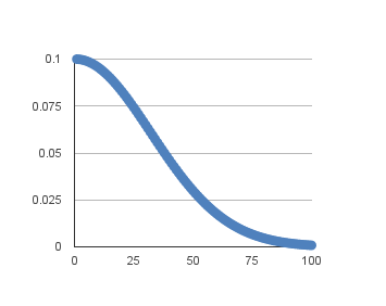
You can create a nice default schedule by setting the decay value as follows:

Decay = LearningRate / Epochs
Decay = 0.1 / 100
Decay = 0.001

The example below demonstrates using the time-based learning rate adaptation schedule in Keras. The learning rate for stochastic gradient descent has been set to a higher value of 0.1. The model is trained for 50 epochs and the decay argument has been set to 0.002, calculated as 0.1/50. Additionally, it can be a good idea to use momentum when using an adaptive learning rate. In this case we use a momentum value of 0.8.

# Time Based Learning Rate Decay
from pandas import read_csv
import numpy
from keras.models import Sequential
from keras.layers import Dense
from keras.optimizers import SGD
from sklearn.preprocessing import LabelEncoder
# fix random seed for reproducibility
seed = 7
numpy.random.seed(seed)
# load dataset
dataframe = read_csv("ionosphere.csv", header=None)
dataset = dataframe.values
# split into input (X) and output (Y) variables
X = dataset[:,0:34].astype(float)
Y = dataset[:,34]
# encode class values as integers
encoder = LabelEncoder()
encoder.fit(Y)
Y = encoder.transform(Y)
# create model
model = Sequential()
model.add(Dense(34, input_dim=34, kernel_initializer='normal', activation='relu'))
model.add(Dense(1, kernel_initializer='normal', activation='sigmoid'))
# Compile model
epochs = 50
learning_rate = 0.1
decay_rate = learning_rate / epochs
momentum = 0.8
sgd = SGD(lr=learning_rate, momentum=momentum, decay=decay_rate, nesterov=False)
model.compile(loss='binary_crossentropy', optimizer=sgd, metrics=['accuracy'])
# Fit the model
model.fit(X, Y, validation_split=0.33, epochs=epochs, batch_size=28, verbose=2)

Drop-Based Learning Rate Schedule

Another popular learning rate schedule used with deep learning models is to systematically drop the learning rate at specific times during training.

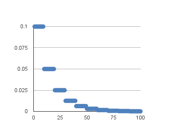
Often this method is implemented by dropping the learning rate by half every fixed number of epochs. For example, we may have an initial learning rate of 0.1 and drop it by 0.5 every 10 epochs. The first 10 epochs of training would use a value of 0.1, in the next 10 epochs a learning rate of 0.05 would be used, and so on.

If we plot out the learning rates for this example out to 100 epochs you get the graph below showing learning rate (y axis) versus epoch (x axis).

We can implement this in Keras using a the LearningRateScheduler callback when fitting the model.

The LearningRateScheduler callback allows us to define a function to call that takes the epoch number as an argument and returns the learning rate to use in stochastic gradient descent. When used, the learning rate specified by stochastic gradient descent is ignored.

In the code below, we use the same example before of a single hidden layer network on the Ionosphere dataset. A new step_decay() function is defined that implements the equation:

LearningRate = InitialLearningRate * DropRate^floor(Epoch / EpochDrop)

Where InitialLearningRate is the initial learning rate such as 0.1, the DropRate is the amount that the learning rate is modified each time it is changed such as 0.5, Epoch is the current epoch number and EpochDrop is how often to change the learning rate such as 10.

Notice that we set the learning rate in the SGD class to 0 to clearly indicate that it is not used. Nevertheless, you can set a momentum term in SGD if you want to use momentum with this learning rate schedule.

# Drop-Based Learning Rate Decay
import pandas
from pandas import read_csv
import numpy
import math
from keras.models import Sequential
from keras.layers import Dense
from keras.optimizers import SGD
from sklearn.preprocessing import LabelEncoder
from keras.callbacks import LearningRateScheduler

# learning rate schedule
def step_decay(epoch):
	initial_lrate = 0.1
	drop = 0.5
	epochs_drop = 10.0
	lrate = initial_lrate * math.pow(drop, math.floor((1+epoch)/epochs_drop))
	return lrate

# fix random seed for reproducibility
seed = 7
numpy.random.seed(seed)
# load dataset
dataframe = read_csv("ionosphere.csv", header=None)
dataset = dataframe.values
# split into input (X) and output (Y) variables
X = dataset[:,0:34].astype(float)
Y = dataset[:,34]
# encode class values as integers
encoder = LabelEncoder()
encoder.fit(Y)
Y = encoder.transform(Y)
# create model
model = Sequential()
model.add(Dense(34, input_dim=34, kernel_initializer='normal', activation='relu'))
model.add(Dense(1, kernel_initializer='normal', activation='sigmoid'))
# Compile model
sgd = SGD(lr=0.0, momentum=0.9, decay=0.0, nesterov=False)
model.compile(loss='binary_crossentropy', optimizer=sgd, metrics=['accuracy'])
# learning schedule callback
lrate = LearningRateScheduler(step_decay)
callbacks_list = [lrate]
# Fit the model
model.fit(X, Y, validation_split=0.33, epochs=50, batch_size=28, callbacks=callbacks_list, verbose=2)

History

History callback records training metrics for each epoch. This includes the loss and the accuracy (for classification problems) as well as the loss and accuracy for the validation dataset, if one is set. The history object is returned from calls to the fit() function used to train the model. Metrics are stored in a dictionary in the history member of the object returned.

For example, you can list the metrics collected in a history object using the following snippet of code after a model is trained:

# list all data in history
print(history.history.keys())

For example, for a model trained on a classification problem with a validation dataset, this might produce the following listing:

['acc', 'loss', 'val_acc', 'val_loss']

Visualize Model Training History in Keras

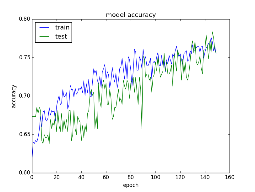
The example collects the history, returned from training the model and creates two charts:

1. A plot of accuracy on the training and validation datasets over training epochs.
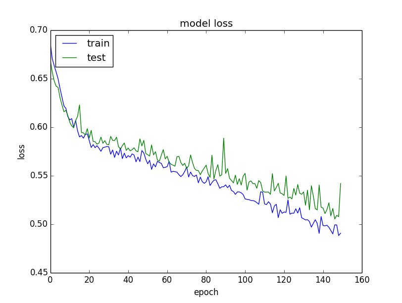
2. A plot of loss on the training and validation datasets over training epochs.

# Visualize training history
from keras.models import Sequential
from keras.layers import Dense
import matplotlib.pyplot as plt
import numpy
# fix random seed for reproducibility
seed = 7
numpy.random.seed(seed)
# load pima indians dataset
dataset = numpy.loadtxt("pima-indians-diabetes.csv", delimiter=",")
# split into input (X) and output (Y) variables
X = dataset[:,0:8]
Y = dataset[:,8]
# create model
model = Sequential()
model.add(Dense(12, input_dim=8, kernel_initializer='uniform', activation='relu'))
model.add(Dense(8, kernel_initializer='uniform', activation='relu'))
model.add(Dense(1, kernel_initializer='uniform', activation='sigmoid'))
# Compile model
model.compile(loss='binary_crossentropy', optimizer='adam', metrics=['accuracy'])
# Fit the model
history = model.fit(X, Y, validation_split=0.33, epochs=150, batch_size=10, verbose=0)
# list all data in history
print(history.history.keys())
# summarize history for accuracy
plt.plot(history.history['acc'])
plt.plot(history.history['val_acc'])
plt.title('model accuracy')
plt.ylabel('accuracy')
plt.xlabel('epoch')
plt.legend(['train', 'test'], loc='upper left')
plt.show()
# summarize history for loss
plt.plot(history.history['loss'])
plt.plot(history.history['val_loss'])
plt.title('model loss')
plt.ylabel('loss')
plt.xlabel('epoch')
plt.legend(['train', 'test'], loc='upper left')
plt.show()

The plots are provided below. The history for the validation dataset is labeled test by convention as it is indeed a test dataset for the model.

From the plot of accuracy we can see that the model could probably be trained a little more as the trend for accuracy on both datasets is still rising for the last few epochs. We can also see that the model has not yet over-learned the training dataset, showing comparable skill on both datasets.

From the plot of loss, we can see that the model has comparable performance on both train and validation datasets (labeled test). If these parallel plots start to depart consistently, it might be a sign to stop training at an earlier epoch.

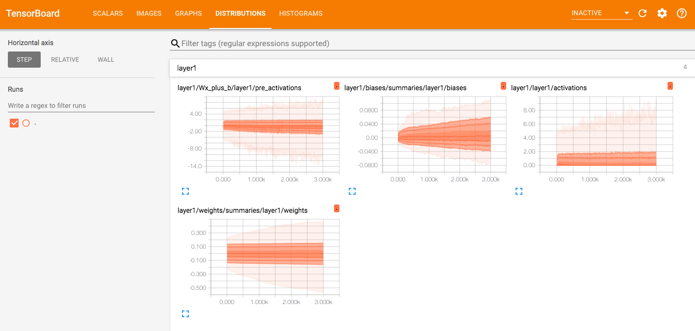
Tensorboard

Visualizing Neuron Weights During Training 如何在使用train_on_batch时候调用tensorboard

def write_to_tensorboard(self,generator_step, summary_writer,losses):

        summary = tf.Summary()

        value = summary.value.add()
        value.simple_value = losses[1]
        value.tag = 'Critic Real Loss'

        value = summary.value.add()
        value.simple_value = losses[2]
        value.tag = 'Critic Fake Loss'

        value = summary.value.add()
        value.simple_value = losses[3]
        value.tag = 'Generator Loss'

        value = summary.value.add()
        value.simple_value = losses[1] - losses[2]
        value.tag = 'Critic Loss (D_real - D_fake)'

        value = summary.value.add()
        value.simple_value = losses[1] + losses[2]
        value.tag = 'Critic Loss (D_fake + D_real)'

        summary_writer.add_summary(summary, generator_step)
        summary_writer.flush()
    def train(self,epochs,batch_size=10,sample_interval=100):
        summary_writer = tf.summary.FileWriter('./logs/trainBoth')
        generator_step = 1

        for epoch in tqdm(range(1, epochs + 1)):
            for e, (figure_imgs, pose_imgs) in tqdm(enumerate(self.data_loader.load_batch(batch_size=batch_size))):
                    # Train the critic

                    figure_loss_real = self.figure_critic.train_on_batch(figure_imgs, valid)
                    figure_loss_fake = self.figure_critic.train_on_batch(gen_figure_imgs, fake)
                    d_figure_loss = 0.5 * np.add(figure_loss_real, figure_loss_fake)

                print(self.figure_critic.metrics_names,d_figure_loss)
                losses = np.empty(shape=1)
                losses = np.append(losses, figure_loss_real)
                losses = np.append(losses, figure_loss_fake)

                # ---------------------
                #  Train Generator
                # ---------------------

                figure_loss = self.figure_EN.train_on_batch([figure_noise,pose_imgs],valid)
                print(self.figure_EN.metrics_names,figure_loss)
                losses = np.append(losses, figure_loss)
                self.write_to_tensorboard(generator_step, summary_writer, losses)
                generator_step += 1

Tensorflow

import tensorflow as tf
from tensorflow.examples.tutorials.mnist import input_data

SUMMARY_DIR = "./graph"
BATCH_SIZE = 100
TRAIN_STEPS = 3000

def variable_summaries(var, name):
    with tf.name_scope('summaries'):
        tf.summary.histogram(name, var)
        mean = tf.reduce_mean(var)
        tf.summary.scalar('mean/' + name, mean)
        stddev = tf.sqrt(tf.reduce_mean(tf.square(var - mean)))
        tf.summary.scalar('stddev/' + name, stddev)

# 2. 生成一层全链接的神经网络
def nn_layer(input_tensor, input_dim, output_dim, layer_name, act=tf.nn.relu):
    with tf.name_scope(layer_name):
        with tf.name_scope('weights'):
            weights = tf.Variable(tf.truncated_normal([input_dim, output_dim], stddev=0.1))
            variable_summaries(weights, layer_name + '/weights')
        with tf.name_scope('biases'):
            biases = tf.Variable(tf.constant(0.0, shape=[output_dim]))
            variable_summaries(biases, layer_name + '/biases')
        with tf.name_scope('Wx_plus_b'):
            preactivate = tf.matmul(input_tensor, weights) + biases
            tf.summary.histogram(layer_name + '/pre_activations', preactivate)
        activations = act(preactivate, name='activation')

        # 记录神经网络节点输出在经过激活函数之后的分布。
        tf.summary.histogram(layer_name + '/activations', activations)
        return activations


def main():
    mnist = input_data.read_data_sets("D:\pyprogram", one_hot=True)

    with tf.name_scope('input'):
        x = tf.placeholder(tf.float32, [None, 784], name='x-input')
        y_ = tf.placeholder(tf.float32, [None, 10], name='y-input')

    with tf.name_scope('input_reshape'):
        image_shaped_input = tf.reshape(x, [-1, 28, 28, 1])
        tf.summary.image('input', image_shaped_input, 10)

    hidden1 = nn_layer(x, 784, 500, 'layer1')
    y = nn_layer(hidden1, 500, 10, 'layer2', act=tf.identity)

    with tf.name_scope('cross_entropy'):
        cross_entropy = tf.reduce_mean(tf.nn.softmax_cross_entropy_with_logits(logits=y, labels=y_))
        tf.summary.scalar('cross_entropy', cross_entropy)

    with tf.name_scope('train'):
        train_step = tf.train.AdamOptimizer(0.001).minimize(cross_entropy)

    with tf.name_scope('accuracy'):
        with tf.name_scope('correct_prediction'):
            correct_prediction = tf.equal(tf.argmax(y, 1), tf.argmax(y_, 1))
        with tf.name_scope('accuracy'):
            accuracy = tf.reduce_mean(tf.cast(correct_prediction, tf.float32))
        tf.summary.scalar('accuracy', accuracy)

    merged = tf.summary.merge_all()

    with tf.Session() as sess:
        summary_writer = tf.summary.FileWriter(SUMMARY_DIR, sess.graph)
        tf.global_variables_initializer().run()

        for i in range(TRAIN_STEPS):
            xs, ys = mnist.train.next_batch(BATCH_SIZE)
            # 运行训练步骤以及所有的日志生成操作，得到这次运行的日志。
            summary, _ = sess.run([merged, train_step], feed_dict={x: xs, y_: ys})
            # 将得到的所有日志写入日志文件，这样TensorBoard程序就可以拿到这次运行所对应的
            # 运行信息。
            summary_writer.add_summary(summary, i)

    summary_writer.close()

if __name__ == '__main__':
    main()

Customerize Optimizer

The following example is an example of modifing the implementation of Adam optimizer, so that it can support differential privacy.

from keras.optimizers import Optimizer
from keras import backend as K


def clip_norm(g, c, n):
    if c > 0:
        g = K.switch(n >= c, g * c / n, g)
    return g


class NoisyAdam(Optimizer):
    def __init__(self, lr=0.001, beta_1=0.9, beta_2=0.999,
                 epsilon=1e-8, decay=0., noise=0., **kwargs):
        super(NoisyAdam, self).__init__(**kwargs)
        self.iterations = K.variable(0, name='iterations')
        self.lr = K.variable(lr, name='lr')
        self.beta_1 = K.variable(beta_1, name='beta_1')
        self.beta_2 = K.variable(beta_2, name='beta_2')
        self.epsilon = epsilon
        self.decay = K.variable(decay, name='decay')
        self.initial_decay = decay
        self.noise = noise

    def get_gradients(self, loss, params):
        grads = K.gradients(loss, params)
        if hasattr(self, 'clipnorm') and self.clipnorm > 0:
            norm = K.sqrt(sum([K.sum(K.square(g)) for g in grads]))
            grads = [clip_norm(g, self.clipnorm, norm) for g in grads]
        if hasattr(self, 'clipvalue') and self.clipvalue > 0:
            grads = [K.clip(g, -self.clipvalue, self.clipvalue) for g in grads]

        if self.noise > 0:
            grads = [(g + K.random_normal(g.shape, mean=0,
                                          stddev=(self.noise * self.clipnorm)))
                     for g in grads]
        return grads

    def get_updates(self, loss,params):
        grads = self.get_gradients(loss, params)
        self.updates = [K.update_add(self.iterations, 1)]

        lr = self.lr
        if self.initial_decay > 0:
            lr *= (1. / (1. + self.decay * self.iterations))

        t = self.iterations + 1
        lr_t = lr * (K.sqrt(1. - K.pow(self.beta_2, t)) /
                     (1. - K.pow(self.beta_1, t)))

        shapes = [K.get_variable_shape(p) for p in params]
        ms = [K.zeros(shape) for shape in shapes]
        vs = [K.zeros(shape) for shape in shapes]
        self.weights = [self.iterations] + ms + vs

        for p, g, m, v in zip(params, grads, ms, vs):
            m_t = (self.beta_1 * m) + (1. - self.beta_1) * g
            v_t = (self.beta_2 * v) + (1. - self.beta_2) * K.square(g)
            p_t = p - lr_t * m_t / (K.sqrt(v_t) + self.epsilon)

            self.updates.append(K.update(m, m_t))
            self.updates.append(K.update(v, v_t))
            new_p = p_t
            # Apply constraints.
            if getattr(p, 'constraint', None) is not None:
                new_p = p.constraint(new_p)

            self.updates.append(K.update(p, new_p))
        return self.updates

    def get_config(self):
        config = {'lr': float(K.get_value(self.lr)),
                  'beta_1': float(K.get_value(self.beta_1)),
                  'beta_2': float(K.get_value(self.beta_2)),
                  'decay': float(K.get_value(self.decay)),
                  'epsilon': self.epsilon}
        base_config = super(NoisyAdam, self).get_config()
        return dict(list(base_config.items()) + list(config.items()))

Feature Extraction

VGG Feature Loss

from keras.applications import VGG19
from keras import layers

def build_vgg():
    vgg = VGG19(weights="imagenet")
    vgg.outputs = [vgg.layers[9].output]
    img = layers.Input(shape=self.img_shape)
    img_features = vgg(img)
    return Model(img, img_features)
##########################################
vgg = build_vgg()
vgg.trainable = False
vgg.compile(loss='mse',optimizer=optimizer,metrics=['accuracy'])

##########################################
fake_pose_vgg_feature = vgg(pose_recons)
pose_ende = Model(pose_img,fake_pose_vgg_feature)
 
##########################################
pose_real_vgg_feature = vgg.predict(pose_imgs)
pose_loss = pose_ende.train_on_batch(pose_imgs,pose_real_vgg_feature)

Fine tune ref

Print Gradients ref

def get_gradients(self,inputs, groundtruth, model):
    opt = model.optimizer
    loss = model.total_loss
    weights = model.weights
    grads = opt.get_gradients(loss, weights)
    grad_fn = K.function(inputs=[model.inputs[0],
                                 model.sample_weights[0],
                                 model.targets[0],
                                 K.learning_phase()],
                         outputs=grads)
    grad_values = grad_fn([inputs, np.ones(len(inputs)), groundtruth, 1])
    return grad_values

Then in the main function:

gradients = self.get_gradients(imgs,valid,self.discriminator)
for i in range(len(gradients)):
    print(i, np.shape(gradients[i]))

HyperparametersSearching

source

# Original Code here:
# https://github.com/pytorch/examples/blob/master/mnist/main.py
from __future__ import print_function

import argparse
import torch
import torch.nn as nn
import torch.nn.functional as F
import torch.optim as optim
from torchvision import datasets, transforms

# Training settings
parser = argparse.ArgumentParser(description="PyTorch MNIST Example")
parser.add_argument(
    "--batch-size",
    type=int,
    default=64,
    metavar="N",
    help="input batch size for training (default: 64)")
parser.add_argument(
    "--test-batch-size",
    type=int,
    default=1000,
    metavar="N",
    help="input batch size for testing (default: 1000)")
parser.add_argument(
    "--epochs",
    type=int,
    default=1,
    metavar="N",
    help="number of epochs to train (default: 1)")
parser.add_argument(
    "--lr",
    type=float,
    default=0.01,
    metavar="LR",
    help="learning rate (default: 0.01)")
parser.add_argument(
    "--momentum",
    type=float,
    default=0.5,
    metavar="M",
    help="SGD momentum (default: 0.5)")
parser.add_argument(
    "--no-cuda",
    action="store_true",
    default=False,
    help="disables CUDA training")
parser.add_argument(
    "--seed",
    type=int,
    default=1,
    metavar="S",
    help="random seed (default: 1)")
parser.add_argument(
    "--smoke-test", action="store_true", help="Finish quickly for testing")


def train_mnist(args, config, reporter):
    vars(args).update(config)
    args.cuda = not args.no_cuda and torch.cuda.is_available()

    torch.manual_seed(args.seed)
    if args.cuda:
        torch.cuda.manual_seed(args.seed)

    kwargs = {"num_workers": 1, "pin_memory": True} if args.cuda else {}
    train_loader = torch.utils.data.DataLoader(
        datasets.MNIST(
            "~/data",
            train=True,
            download=False,
            transform=transforms.Compose([
                transforms.ToTensor(),
                transforms.Normalize((0.1307, ), (0.3081, ))
            ])),
        batch_size=args.batch_size,
        shuffle=True,
        **kwargs)
    test_loader = torch.utils.data.DataLoader(
        datasets.MNIST(
            "~/data",
            train=False,
            transform=transforms.Compose([
                transforms.ToTensor(),
                transforms.Normalize((0.1307, ), (0.3081, ))
            ])),
        batch_size=args.test_batch_size,
        shuffle=True,
        **kwargs)

    class Net(nn.Module):
        def __init__(self):
            super(Net, self).__init__()
            self.conv1 = nn.Conv2d(1, 10, kernel_size=5)
            self.conv2 = nn.Conv2d(10, 20, kernel_size=5)
            self.conv2_drop = nn.Dropout2d()
            self.fc1 = nn.Linear(320, 50)
            self.fc2 = nn.Linear(50, 10)

        def forward(self, x):
            x = F.relu(F.max_pool2d(self.conv1(x), 2))
            x = F.relu(F.max_pool2d(self.conv2_drop(self.conv2(x)), 2))
            x = x.view(-1, 320)
            x = F.relu(self.fc1(x))
            x = F.dropout(x, training=self.training)
            x = self.fc2(x)
            return F.log_softmax(x, dim=1)

    model = Net()
    if args.cuda:
        model.cuda()

    optimizer = optim.SGD(
        model.parameters(), lr=args.lr, momentum=args.momentum)

    def train(epoch):
        model.train()
        for batch_idx, (data, target) in enumerate(train_loader):
            if args.cuda:
                data, target = data.cuda(), target.cuda()
            optimizer.zero_grad()
            output = model(data)
            loss = F.nll_loss(output, target)
            loss.backward()
            optimizer.step()

    def test():
        model.eval()
        test_loss = 0
        correct = 0
        with torch.no_grad():
            for data, target in test_loader:
                if args.cuda:
                    data, target = data.cuda(), target.cuda()
                output = model(data)
                # sum up batch loss
                test_loss += F.nll_loss(output, target, reduction="sum").item()
                # get the index of the max log-probability
                pred = output.argmax(dim=1, keepdim=True)
                correct += pred.eq(
                    target.data.view_as(pred)).long().cpu().sum()

        test_loss = test_loss / len(test_loader.dataset)
        accuracy = correct.item() / len(test_loader.dataset)
        reporter(mean_loss=test_loss, mean_accuracy=accuracy)

    for epoch in range(1, args.epochs + 1):
        train(epoch)
        test()


if __name__ == "__main__":
    datasets.MNIST("~/data", train=True, download=True)
    args = parser.parse_args()

    import numpy as np
    import ray
    from ray import tune
    from ray.tune.schedulers import AsyncHyperBandScheduler

    ray.init()
    sched = AsyncHyperBandScheduler(
        time_attr="training_iteration",
        reward_attr="neg_mean_loss",
        max_t=400,
        grace_period=20)
    tune.register_trainable(
        "TRAIN_FN",
        lambda config, reporter: train_mnist(args, config, reporter))
    tune.run(
        "TRAIN_FN",
        name="exp",
        scheduler=sched,
        **{
            "stop": {
                "mean_accuracy": 0.98,
                "training_iteration": 1 if args.smoke_test else 20
            },
            "resources_per_trial": {
                "cpu": 3,
                "gpu": int(not args.no_cuda)
            },
            "num_samples": 1 if args.smoke_test else 10,
            "config": {
                "lr": tune.sample_from(
                    lambda spec: np.random.uniform(0.001, 0.1)),
                "momentum": tune.sample_from(
                    lambda spec: np.random.uniform(0.1, 0.9)),
            }
        })