Training Techiniques

Techniques for training a Deep Learning model.

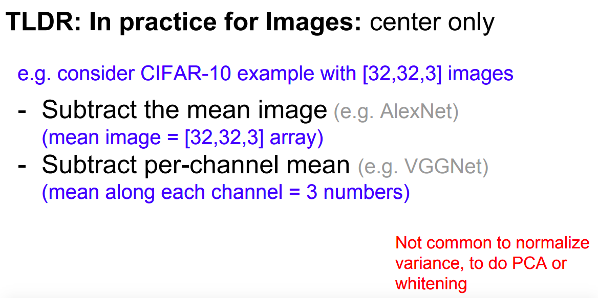
Data Preprocessing

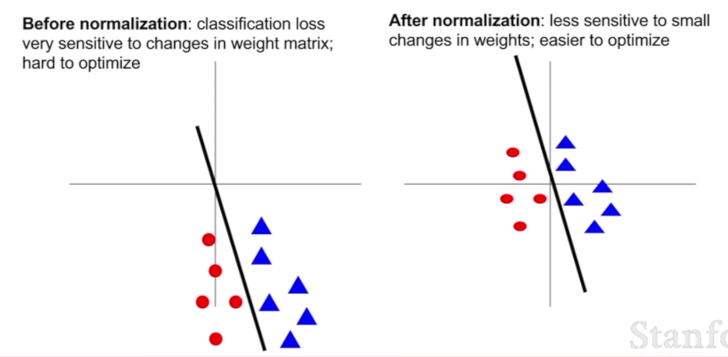
Say we have a binary classification problem where we want to draw a line to separate these red points from these blue points, like the following picture. On the left, thses data points are not normalized and not centered and far away from the origion, although we can still use a line to seperate them, if that line wiggles just a little bit, then our classification is going to get totally destroyed. That kind of means that in the example on the left, the loss function is now extremely sensitive to small perturbations in that linear classifier in our weight matrix. We can still represent the same functions, but that might make learning quite difficult.

On the right situation, if you take the data cloud and move it into the origin and you make it unit variance, then now again, we can still classfiy that data quite well, but now as we wiggle that line a little bit, our loss function is less sensitive to small perturbations in the parameter values. That maybe makes optimization a little bit easier.

Soft labels

This is extremely important when training the discriminator. Having hard labels (1 or 0) nearly killed all learning early on, leading the discriminator to approach 0 loss very rapidly. I ended up using a random number between 0 and 0.1 to represent 0 labels (real images) and a random number between 0.9 and 1.0 to represent 1 labels (generated images). This is not required when training the generator. resource

valid = np.random.uniform(0.9,1.0,size=(batch_size,1))
fake = np.random.uniform(0,0.1,size=(batch_size,1))

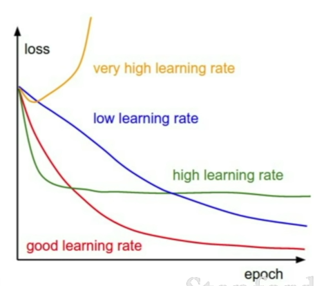
Learning Rate

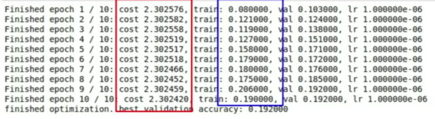
Loss not going down: learning rate is too low

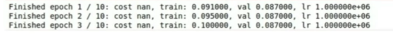
Loss exploding: learning rate too high

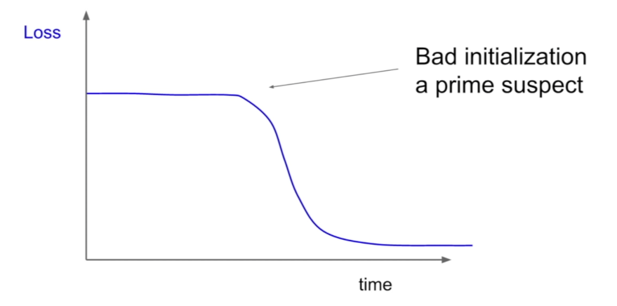
Weight Initialization

Problem with initializing all weights to 0

In this case, the equations of the learning algorithm would fail to make any changes to the network weights, and the model will be stuck. It is important to note that the bias weight in each neuron is set to zero by default, not a small random value. ref

During forward propagation each unit in hidden layer gets signal:

That is, each hidden unit gets sum of inputs multiplied by the corresponding weight.

Now imagine that you initialize all weights to the same value (e.g. zero or one). In this case, each hidden unit will get exactly the same signal. E.g. if all weights are initialized to 1, each unit gets signal equal to sum of inputs (and outputs sigmoid(sum(inputs))). If all weights are zeros, which is even worse, every hidden unit will get zero signal. No matter what was the input - if all weights are the same, all units in hidden layer will be the same too.

This is the main issue with symmetry and reason why you should initialize weights randomly (or, at least, with different values). Note, that this issue affects all architectures that use each-to-each connections. ref

Problems with initializing weights randomly ref

Vanishing gradients

If weights are initialized with low values it gets mapped to 0, then the activation value would be small, say, almost 0. When backpropogating gradients, samll gradients times small weights, it will result in smaller gradients, meaning the earlier layers, the samller gradients, resulting vanishing gradients.

Exploding gradients

Consider you have non-negative and large weights and small activations A (as can be the case for sigmoid(z)). When these weights are multiplied along the layers, they cause a large change in the cost. Thus, the gradients are also going to be large. This means that the changes in W, by W — ⍺ * dW, will be in huge steps, the downward moment will increase.

This may result in oscillating around the minima or even overshooting the optimum again and again and the model will never learn!

Another impact of exploding gradients is that huge values of the gradients may cause number overflow resulting in incorrect computations or introductions of NaN’s. This might also lead to the loss taking the value NaN.

New Initialization techniques ref

Xavier initialization

It is used when we use tanh as our activation function.

Some also use the following as initialization:

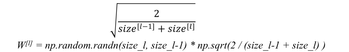
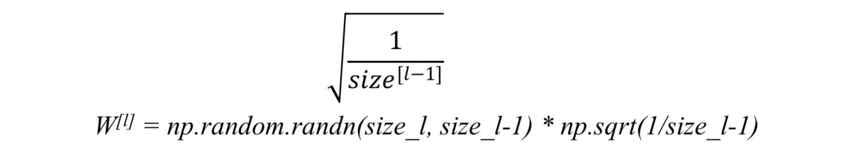
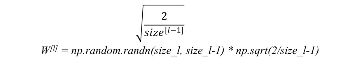
He initialization

When we use relu as activation, we just simply multiply random initialization with:

Batch Normalization

Motivation

Machine learning methods tend to work better when their input data consists of uncorrelated features with zero mean and unit variance. When training a neural network, we can preprocess the data before feeding it to the network to explicitly decorrelate its features; this will ensure that the first layer of the network sees data that follows a nice distribution. However, even if we preprocess the input data, the activations at deeper layers of the network will likely no longer be decorrelated and will no longer have zero mean or unit variance since they are output from earlier layers in the network. Even worse, during the training process the distribution of features at each layer of the network will shift as the weights of each layer are updated.

The authors of [1] hypothesize that the shifting distribution of features inside deep neural networks may make training deep networks more difficult. To overcome this problem, [1] proposes to insert batch normalization layers into the network. At training time, a batch normalization layer uses a minibatch of data to estimate the mean and standard deviation of each feature. These estimated means and standard deviations are then used to center and normalize the features of the minibatch. A running average of these means and standard deviations is kept during training, and at test time these running averages are used to center and normalize features.

It is possible that this normalization strategy could reduce the representational power of the network, since it may sometimes be optimal for certain layers to have features that are not zero-mean or unit variance. To this end, the batch normalization layer includes learnable shift and scale parameters for each feature dimension. [cs231n]

Usually, in order to train a neural network, we do some preprocessing to the input data. For example, we could normalize all data (whitening) so that it resembles a normal distribution (that means, zero mean and a unitary variance). Why do we do this preprocessing? Well, there are many reasons for that, some of them being: preventing the early saturation of non-linear activation functions like the sigmoid function, assuring that all input data is in the same range of values, etc.

But the problem appears in the intermediate layers because the distribution of the activations is constantly changing during training. This slows down the training process because each layer must learn to adapt themselves to a new distribution in every training step. This problem is known as internal covariate shift.

So… what happens if we force the input of every layer to have approximately the same distribution in every training step? ref

BN的基本思想其实相当直观：因为深层神经网络在做非线性变换前的激活输入值（就是那个x=WU+B，U是输入）随着网络深度加深或者在训练过程中，其分布逐渐发生偏移或者变动，之所以训练收敛慢，一般是整体分布逐渐往非线性函数的取值区间的上下限两端靠近（对于Sigmoid函数来说，意味着激活输入值WU+B是大的负值或正值），所以这导致反向传播时低层神经网络的梯度消失，这是训练深层神经网络收敛越来越慢的本质原因，而BN就是通过一定的规范化手段，把每层神经网络任意神经元这个输入值的分布强行拉回到均值为0方差为1的标准正态分布，其实就是把越来越偏的分布强制拉回比较标准的分布，这样使得激活输入值落在非线性函数对输入比较敏感的区域，这样输入的小变化就会导致损失函数较大的变化，意思是这样让梯度变大，避免梯度消失问题产生，而且梯度变大意味着学习收敛速度快，能大大加快训练速度。 ref

Method

Batch normalization is a method we can use to normalize the inputs of each layer, in order to fight the internal covariate shift problem.

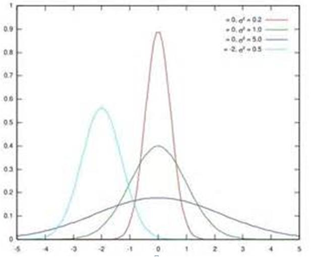
假设某个隐层神经元原先的激活输入x取值符合正态分布，正态分布均值是-2，方差是0.5，对应上图中最左端的浅蓝色曲线，通过BN后转换为均值为0，方差是1的正态分布（对应上图中的深蓝色图形），意味着什么，意味着输入x的取值正态分布整体右移2（均值的变化），图形曲线更平缓了（方差增大的变化）。这个图的意思是，BN其实就是把每个隐层神经元的激活输入分布从偏离均值为0方差为1的正态分布通过平移均值压缩或者扩大曲线尖锐程度，调整为均值为0方差为1的正态分布。

　　那么把激活输入x调整到这个正态分布有什么用？首先我们看下均值为0，方差为1的标准正态分布代表什么含义：

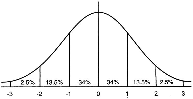
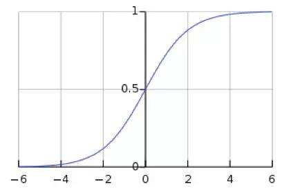
这意味着在一个标准差范围内，也就是说64%的概率x其值落在[-1,1]的范围内，在两个标准差范围内，也就是说95%的概率x其值落在了[-2,2]的范围内。那么这又意味着什么？我们知道，激活值x=WU+B,U是真正的输入，x是某个神经元的激活值，假设非线性函数是sigmoid，那么看下sigmoid(x)其图形：

及sigmoid(x)的导数为：G’=f(x)*(1-f(x))，因为f(x)=sigmoid(x)在0到1之间，所以G’在0到0.25之间，其对应的图如下：

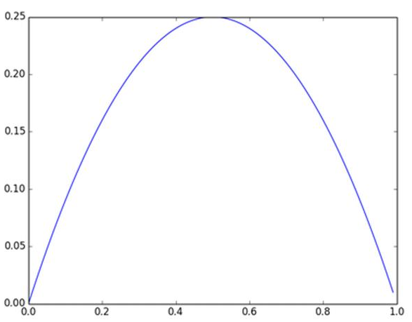
假设没有经过BN调整前x的原先正态分布均值是-6，方差是1，那么意味着95%的值落在了[-8,-4]之间，那么对应的Sigmoid（x）函数的值明显接近于0，这是典型的梯度饱和区，在这个区域里梯度变化很慢，为什么是梯度饱和区？请看下sigmoid(x)如果取值接近0或者接近于1的时候对应导数函数取值，接近于0，意味着梯度变化很小甚至消失。而假设经过BN后，均值是0，方差是1，那么意味着95%的x值落在了[-2,2]区间内，很明显这一段是sigmoid(x)函数接近于线性变换的区域，意味着x的小变化会导致非线性函数值较大的变化，也即是梯度变化较大，对应导数函数图中明显大于0的区域，就是梯度非饱和区。

　　从上面几个图应该看出来BN在干什么了吧？其实就是把隐层神经元激活输入x=WU+B从变化不拘一格的正态分布通过BN操作拉回到了均值为0，方差为1的正态分布，即原始正态分布中心左移或者右移到以0为均值，拉伸或者缩减形态形成以1为方差的图形。什么意思？就是说经过BN后，目前大部分Activation的值落入非线性函数的线性区内，其对应的导数远离导数饱和区，这样来加速训练收敛过程。

　　但是很明显，看到这里，稍微了解神经网络的读者一般会提出一个疑问：如果都通过BN，那么不就跟把非线性函数替换成线性函数效果相同了？这意味着什么？我们知道，如果是多层的线性函数变换其实这个深层是没有意义的，因为多层线性网络跟一层线性网络是等价的。这意味着网络的表达能力下降了，这也意味着深度的意义就没有了。所以BN为了保证非线性的获得，对变换后的满足均值为0方差为1的x又进行了scale加上shift操作(y=scale*x+shift)，每个神经元增加了两个参数scale和shift参数，这两个参数是通过训练学习到的，意思是通过scale和shift把这个值从标准正态分布左移或者右移一点并长胖一点或者变瘦一点，每个实例挪动的程度不一样，这样等价于非线性函数的值从正中心周围的线性区往非线性区动了动。核心思想应该是想找到一个线性和非线性的较好平衡点，既能享受非线性的较强表达能力的好处，又避免太靠非线性区两头使得网络收敛速度太慢。当然，这是我的理解，论文作者并未明确这样说。但是很明显这里的scale和shift操作是会有争议的，因为按照论文作者论文里写的理想状态，就会又通过scale和shift操作把变换后的x调整回未变换的状态，那不是饶了一圈又绕回去原始的“Internal Covariate Shift”问题里去了吗，感觉论文作者并未能够清楚地解释scale和shift操作的理论原因。

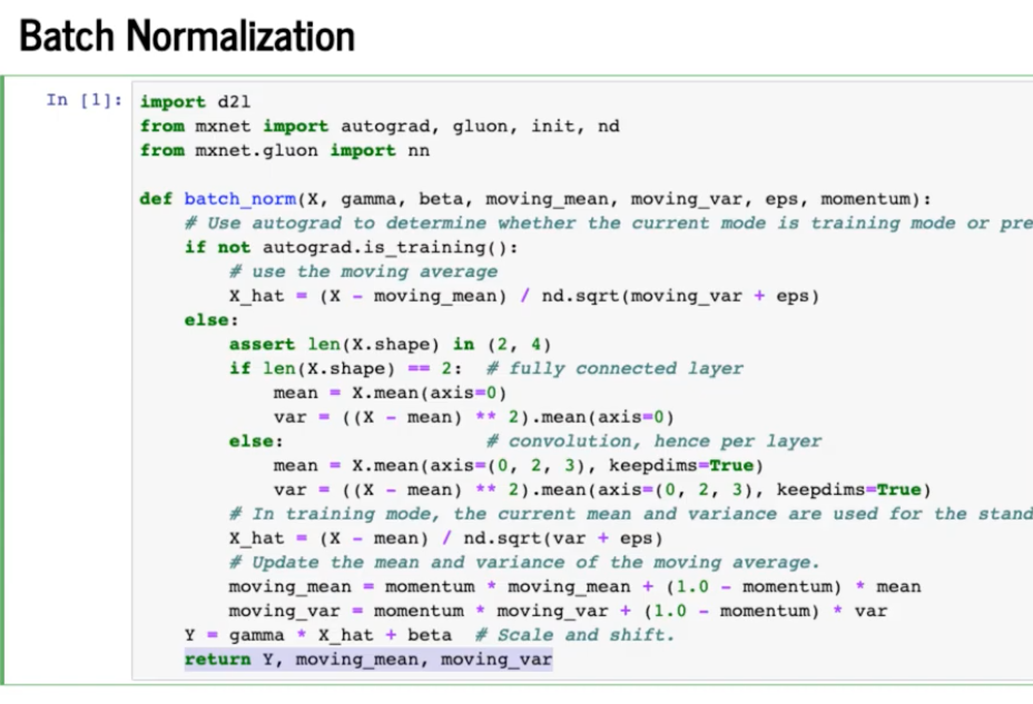
训练阶段如何做BatchNorm

上面是对BN的抽象分析和解释，具体在Mini-Batch SGD下做BN怎么做？其实论文里面这块写得很清楚也容易理解。为了保证这篇文章完整性，这里简单说明下。

　　假设对于一个深层神经网络来说，其中两层结构如下：

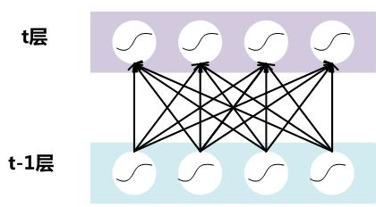
要对每个隐层神经元的激活值做BN，可以想象成每个隐层又加上了一层BN操作层，它位于X=WU+B激活值获得之后，非线性函数变换之前，其图示如下：

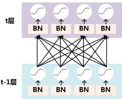
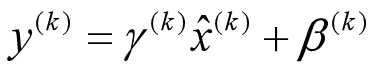
对于Mini-Batch SGD来说，一次训练过程里面包含m个训练实例，其具体BN操作就是对于隐层内每个神经元的激活值来说，进行如下变换：

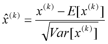
要注意，这里t层某个神经元的x(k)不是指原始输入，就是说不是t-1层每个神经元的输出，而是t层这个神经元的线性激活x=WU+B，这里的U才是t-1层神经元的输出。变换的意思是：某个神经元对应的原始的激活x通过减去mini-Batch内m个实例获得的m个激活x求得的均值E(x)并除以求得的方差Var(x)来进行转换。

　　上文说过经过这个变换后某个神经元的激活x形成了均值为0，方差为1的正态分布，目的是把值往后续要进行的非线性变换的线性区拉动，增大导数值，增强反向传播信息流动性，加快训练收敛速度。但是这样会导致网络表达能力下降，为了防止这一点，每个神经元增加两个调节参数（scale和shift），这两个参数是通过训练来学习到的，用来对变换后的激活反变换，使得网络表达能力增强，即对变换后的激活进行如下的scale和shift操作，这其实是变换的反操作：

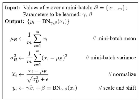
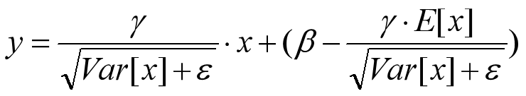
Look at the last line of the algorithm. After normalizing the input x the result is squashed through a linear function with parameters gamma and beta. These are learnable parameters of the BatchNorm Layer and make it basically possible to say “Hey!! I don’t want zero mean/unit variance input, give me back the raw input - it’s better for me.” If gamma = sqrt(var(x)) and beta = mean(x), the original activation is restored. This is, what makes BatchNorm really powerful. We initialize the BatchNorm Parameters to transform the input to zero mean/unit variance distributions but during training they can learn that any other distribution might be better.

Btw: it’s called “Batch” Normalization because we perform this transformation and calculate the statistics only for a subpart (a batch) of the entire training set. source

BatchNorm的推理(Inference)过程

BN在训练的时候可以根据Mini-Batch里的若干训练实例进行激活数值调整，但是在推理（inference）的过程中，很明显输入就只有一个实例，看不到Mini-Batch其它实例，那么这时候怎么对输入做BN呢？因为很明显一个实例是没法算实例集合求出的均值和方差的。这可如何是好？

　　既然没有从Mini-Batch数据里可以得到的统计量，那就想其它办法来获得这个统计量，就是均值和方差。可以用从所有训练实例中获得的统计量来代替Mini-Batch里面m个训练实例获得的均值和方差统计量，因为本来就打算用全局的统计量，只是因为计算量等太大所以才会用Mini-Batch这种简化方式的，那么在推理的时候直接用全局统计量即可。

　　决定了获得统计量的数据范围，那么接下来的问题是如何获得均值和方差的问题。很简单，因为每次做Mini-Batch训练时，都会有那个Mini-Batch里m个训练实例获得的均值和方差，现在要全局统计量，只要把每个Mini-Batch的均值和方差统计量记住，然后对这些均值和方差求其对应的数学期望即可得出全局统计量，即：

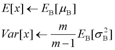
有了均值和方差，每个隐层神经元也已经有对应训练好的Scaling参数和Shift参数，就可以在推导的时候对每个神经元的激活数据计算NB进行变换了，在推理过程中进行BN采取如下方式：

这个公式其实和训练时

是等价的，通过简单的合并计算推导就可以得出这个结论。那么为啥要写成这个变换形式呢？我猜作者这么写的意思是：在实际运行的时候，按照这种变体形式可以减少计算量，为啥呢？因为对于每个隐层节点来说：

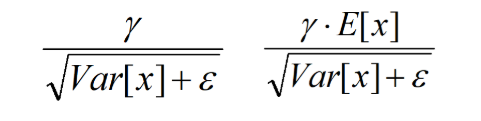
都是固定值，这样这两个值可以事先算好存起来，在推理的时候直接用就行了，这样比原始的公式每一步骤都现算少了除法的运算过程，乍一看也没少多少计算量，但是如果隐层节点个数多的话节省的计算量就比较多了。

BatchNorm的好处

BatchNorm为什么NB呢，关键还是效果好。①**不仅仅极大提升了训练速度，收敛过程大大加快；②还能增加分类效果，一种解释是这是类似于Dropout的一种防止过拟合的正则化表达方式，所以不用Dropout也能达到相当的效果；③另外调参过程也简单多了，对于初始化要求没那么高，而且可以使用大的学习率等。**总而言之，经过这么简单的变换，带来的好处多得很，这也是为何现在BN这么快流行起来的原因。

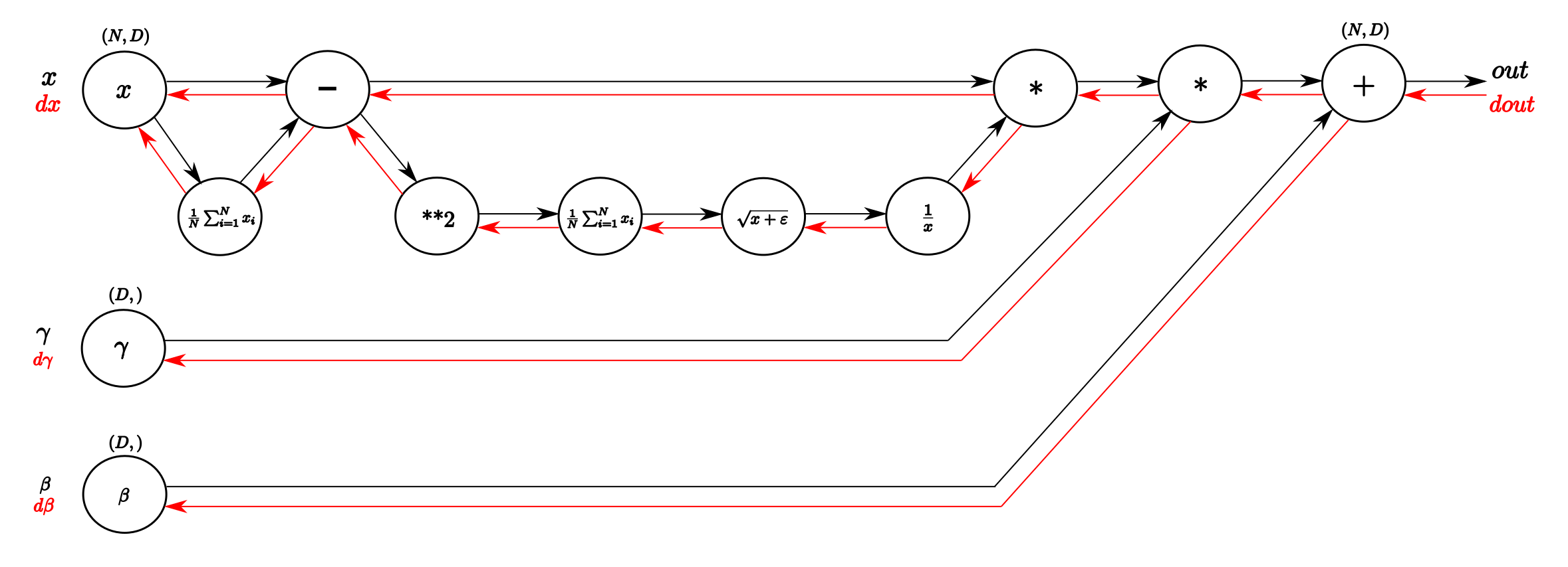
Implementation

Forward

def batchnorm_forward(x, gamma, beta, bn_param):
    """
    Forward pass for batch normalization.

    During training the sample mean and (uncorrected) sample variance are
    computed from minibatch statistics and used to normalize the incoming data.
    During training we also keep an exponentially decaying running mean of the
    mean and variance of each feature, and these averages are used to normalize
    data at test-time.

    At each timestep we update the running averages for mean and variance using
    an exponential decay based on the momentum parameter:

    running_mean = momentum * running_mean + (1 - momentum) * sample_mean
    running_var = momentum * running_var + (1 - momentum) * sample_var

    Note that the batch normalization paper suggests a different test-time
    behavior: they compute sample mean and variance for each feature using a
    large number of training images rather than using a running average. For
    this implementation we have chosen to use running averages instead since
    they do not require an additional estimation step; the torch7
    implementation of batch normalization also uses running averages.

    Input:
    - x: Data of shape (N, D)
    - gamma: Scale parameter of shape (D,)
    - beta: Shift paremeter of shape (D,)
    - bn_param: Dictionary with the following keys:
      - mode: 'train' or 'test'; required
      - eps: Constant for numeric stability
      - momentum: Constant for running mean / variance.
      - running_mean: Array of shape (D,) giving running mean of features
      - running_var Array of shape (D,) giving running variance of features

    Returns a tuple of:
    - out: of shape (N, D)
    - cache: A tuple of values needed in the backward pass
    """
    mode = bn_param['mode']
    eps = bn_param.get('eps', 1e-5)
    momentum = bn_param.get('momentum', 0.9)

    N, D = x.shape
    running_mean = bn_param.get('running_mean', np.zeros(D, dtype=x.dtype))
    running_var = bn_param.get('running_var', np.zeros(D, dtype=x.dtype))

    out, cache = None, None
    if mode == 'train':
        #######################################################################
        # TODO: Implement the training-time forward pass for batch norm.      #
        # Use minibatch statistics to compute the mean and variance, use      #
        # these statistics to normalize the incoming data, and scale and      #
        # shift the normalized data using gamma and beta.                     #
        #                                                                     #
        # You should store the output in the variable out. Any intermediates  #
        # that you need for the backward pass should be stored in the cache   #
        # variable.                                                           #
        #                                                                     #
        # You should also use your computed sample mean and variance together #
        # with the momentum variable to update the running mean and running   #
        # variance, storing your result in the running_mean and running_var   #
        # variables.                                                          #
        #                                                                     #
        # Note that though you should be keeping track of the running         #
        # variance, you should normalize the data based on the standard       #
        # deviation (square root of variance) instead!                        # 
        # Referencing the original paper (https://arxiv.org/abs/1502.03167)   #
        # might prove to be helpful.                                          #
        #######################################################################
        # *****START OF YOUR CODE (DO NOT DELETE/MODIFY THIS LINE)*****

        sample_mean = np.mean(x,axis=0)
        sample_var = np.var(x,axis=0)
        x_hat = (x-sample_mean)/np.sqrt(sample_var+eps)
        out = gamma*x_hat + beta
        
        running_mean = momentum * running_mean + (1 - momentum) * sample_mean
        running_var = momentum * running_var + (1 - momentum) * sample_var
        
        cache = (x,sample_mean,sample_var,x_hat,out,gamma,beta,eps)

        # *****END OF YOUR CODE (DO NOT DELETE/MODIFY THIS LINE)*****
        #######################################################################
        #                           END OF YOUR CODE                          #
        #######################################################################
    elif mode == 'test':
        #######################################################################
        # TODO: Implement the test-time forward pass for batch normalization. #
        # Use the running mean and variance to normalize the incoming data,   #
        # then scale and shift the normalized data using gamma and beta.      #
        # Store the result in the out variable.                               #
        #######################################################################
        # *****START OF YOUR CODE (DO NOT DELETE/MODIFY THIS LINE)*****

        out = gamma*(x-running_mean)/np.sqrt(running_var+eps) + beta

        # *****END OF YOUR CODE (DO NOT DELETE/MODIFY THIS LINE)*****
        #######################################################################
        #                          END OF YOUR CODE                           #
        #######################################################################
    else:
        raise ValueError('Invalid forward batchnorm mode "%s"' % mode)

    # Store the updated running means back into bn_param
    bn_param['running_mean'] = running_mean
    bn_param['running_var'] = running_var

    return out, cache

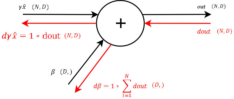
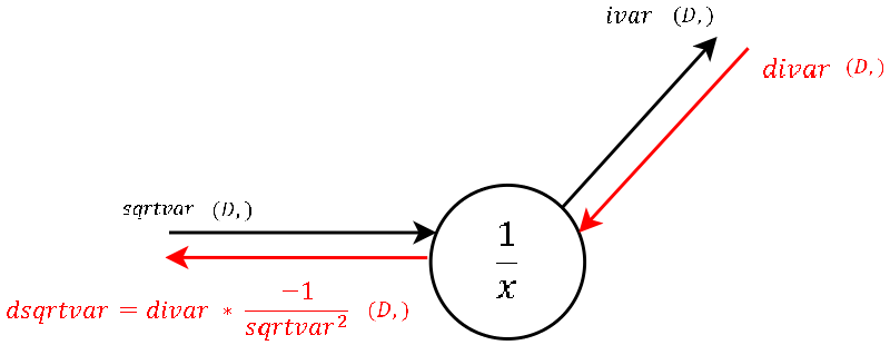
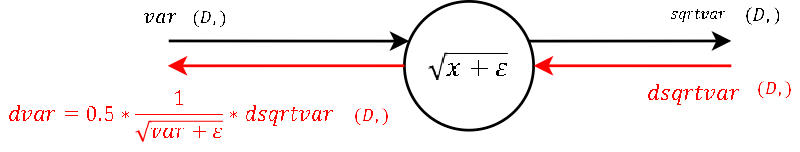
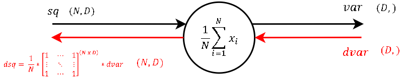
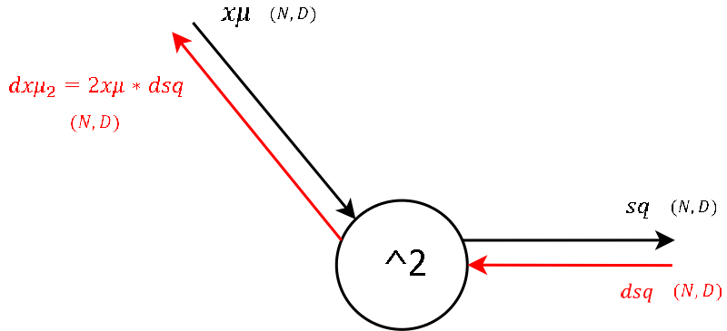
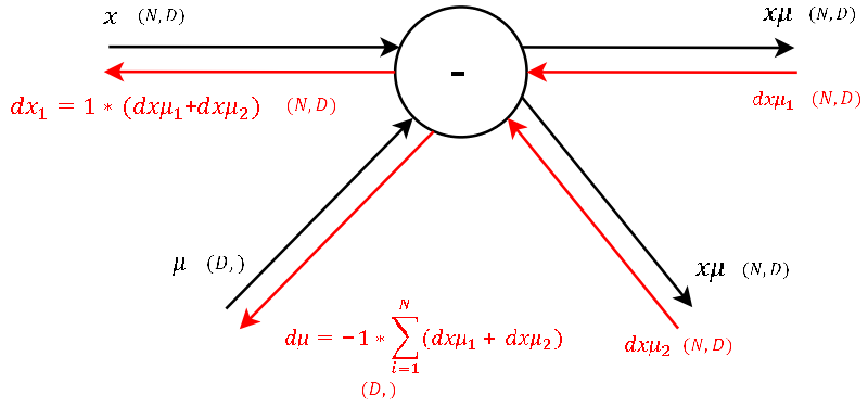
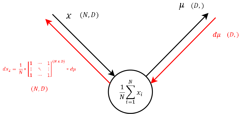
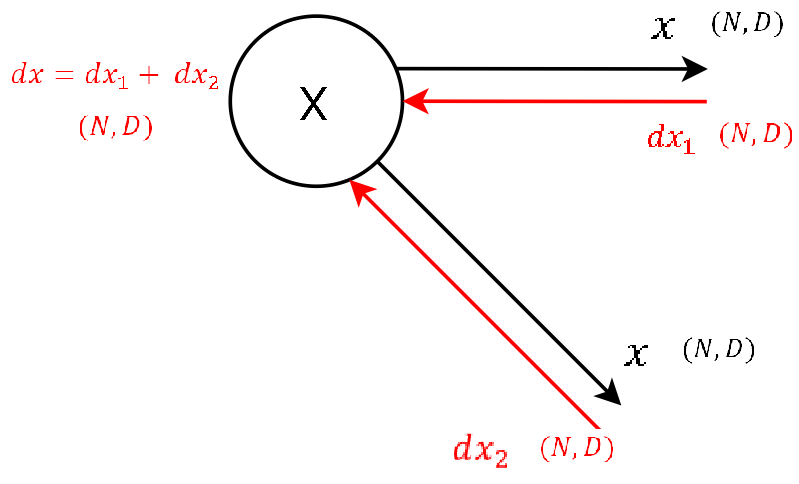
Navie Backward

Step 9

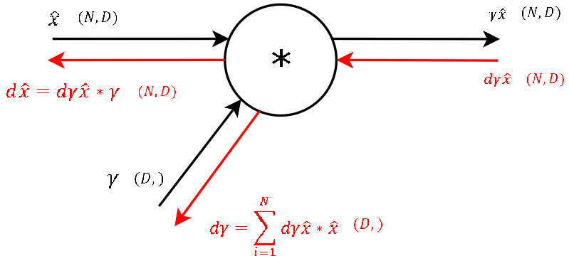
Step 8

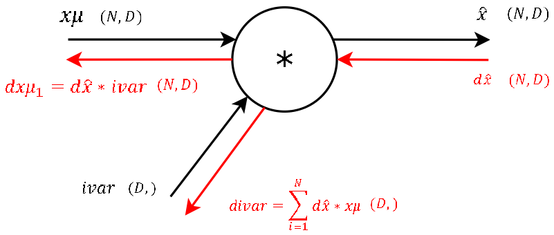
Step 7

Step 6

Step 5

Step 4

Step 3

Step 2

Step 1

Step 0

def batchnorm_backward(dout, cache):
    """
    Backward pass for batch normalization.

    For this implementation, you should write out a computation graph for
    batch normalization on paper and propagate gradients backward through
    intermediate nodes.

    Inputs:
    - dout: Upstream derivatives, of shape (N, D)
    - cache: Variable of intermediates from batchnorm_forward.

    Returns a tuple of:
    - dx: Gradient with respect to inputs x, of shape (N, D)
    - dgamma: Gradient with respect to scale parameter gamma, of shape (D,)
    - dbeta: Gradient with respect to shift parameter beta, of shape (D,)
    """
    
    dx, dgamma, dbeta = None, None, None
    ###########################################################################
    # TODO: Implement the backward pass for batch normalization. Store the    #
    # results in the dx, dgamma, and dbeta variables.                         #
    # Referencing the original paper (https://arxiv.org/abs/1502.03167)       #
    # might prove to be helpful.                                              #
    ###########################################################################
    # *****START OF YOUR CODE (DO NOT DELETE/MODIFY THIS LINE)*****
    N,D = dout.shape
    (x,sample_mean,sample_var,x_hat,out,gamma,beta,eps) = cache
    
    dbeta = np.sum(dout,axis=0)
    dgamma = np.sum(x_hat*dout,axis=0)
    dx_hat = dout*gamma
    
    ivar = 1/np.sqrt(sample_var+eps)
    xmu = x-sample_mean
    
    dx_xmu1 = dx_hat*ivar 
    divar = np.sum(dx_hat*xmu,axis=0)
    
    dsqrt_var = -1*divar/(sample_var+eps)
    
    dvar = 0.5*dsqrt_var/np.sqrt(sample_var+eps)
    
    dsq = np.ones((N,D))*dvar/N
    
    dx_xmu2 = 2*xmu*dsq
    
    dx1 = dx_xmu1 + dx_xmu2
    dmu = -1*np.sum(dx_xmu1 + dx_xmu2,axis=0)
    
    dx2 = np.ones((N,D))*dmu/N
    
    dx = dx1+dx2
    
    # *****END OF YOUR CODE (DO NOT DELETE/MODIFY THIS LINE)*****
    ###########################################################################
    #                             END OF YOUR CODE                            #
    ###########################################################################

    return dx, dgamma, dbeta

Alternative Backward

激活函数

ref1 zhihu intuition details to do

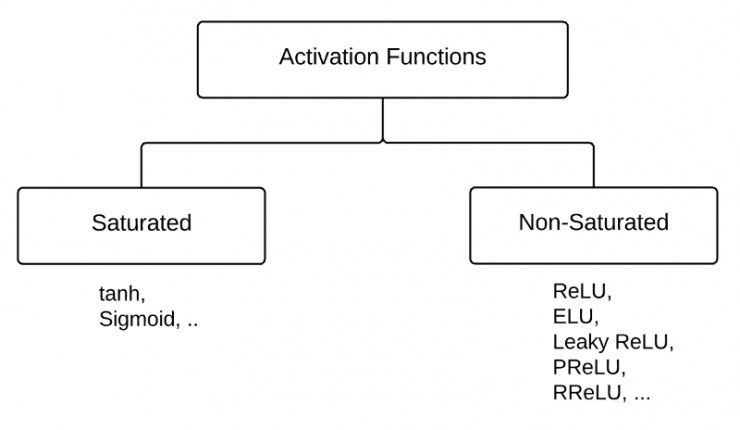
根据是否饱和，激活函数可以分类为“饱和激活函数”和“非饱和激活函数”。

sigmoid和tanh是“饱和激活函数”，而ReLU及其变体则是“非饱和激活函数”，但是他们都属于非线性激活函数。使用“非饱和激活函数”的优势在于两点：

1.首先，“非饱和激活函数”能解决所谓的“梯度消失”问题。 vanishing gradient在网络层数多的时候尤其明显，是加深网络结构的主要障碍之一

2.其次，它能加快收敛速度。

Sigmoid函数

将实数压缩到$(0,1)$，用来二分类。

$$f(x) = \frac{1}{1+e^{-x}}$$

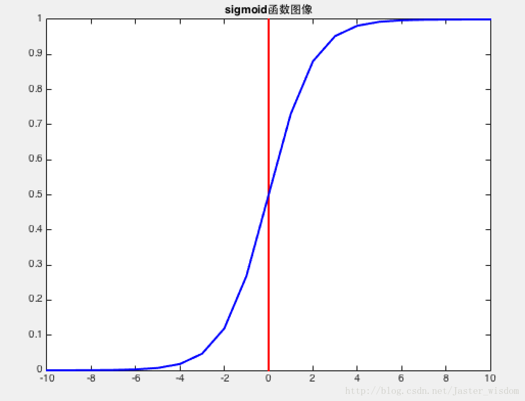
sigmoid的优缺点source

• Vanishing gradients: Notice, the sigmoid function is flat near 0 and 1. In other words, the gradient of the sigmoid is near 0 and 1. During backpropagation through the network with sigmoid activation, the gradients in neurons whose output is near 0 or 1 are nearly 0. These neurons are called saturated neurons. Thus, the weights in these neurons do not update. Not only that, the weights of neurons connected to such neurons are also slowly updated. This problem is also known as vanishing gradient. So, imagine if there was a large network comprising of sigmoid neurons in which many of them are in a saturated regime, then the network will not be able to backpropagate.

  ref1 在GAN中， 给 D 最后的输出加个 Sigmoid 激活函数，让它取值在 0 到 1 之间？事实上这个方案在理论上是没有问题的，然而这会造成训练的困难。因为 Sigmoid 函数具有饱和区，一旦 D 进入了饱和区，就很难传回梯度来更新 G 了。

• Not zero centered: Sigmoid outputs are not zero-centered. The output is always between 0 and 1, that means that the output after applying sigmoid is always positive hence, i.e. $x_i > 0$.

  

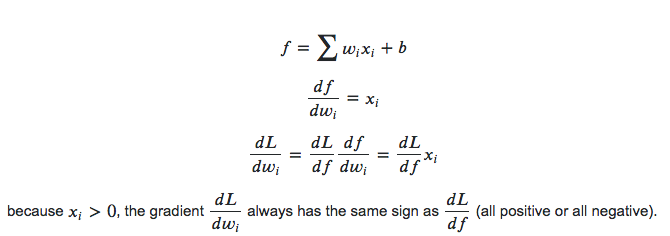
  which means the gradients on the weights $w$ during backpropagation become either all positive or all negative. This could introduce undesirable zig-zagging dynamics in the gradient updates for the weights. Say we

  • Tanh, Rectified Linear Unit (ReLU), Leaky ReLU and Parametric ReLU are all zero-centered activation functions.
  • This is also why you want zero-mean data

• Computationally expensive: The exp() function is computationally expensive compared with the other non-linear activation functions.

Tanh函数

将实数压缩到$[-1,1]$

$$f(x) = tanh(x)=\frac{e^x-e^{-x}}{e^x+e^{-x}}\\ f'(x)=1-f^2(x)$$

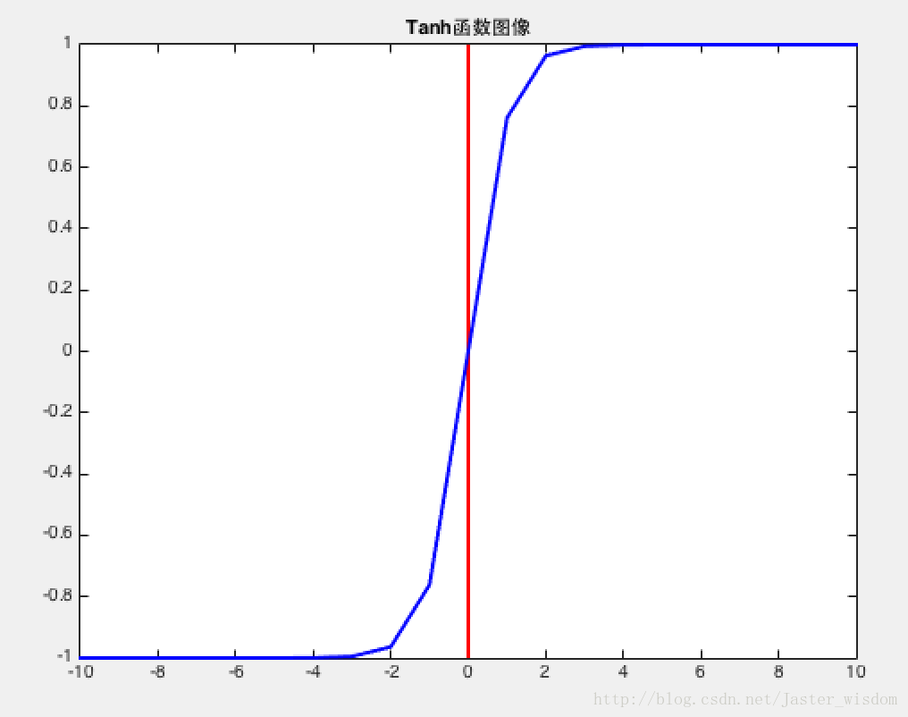
ZERO-centered but still kills gradients when saturated

ReLu函数

$$f(x)=max(0,x)$$

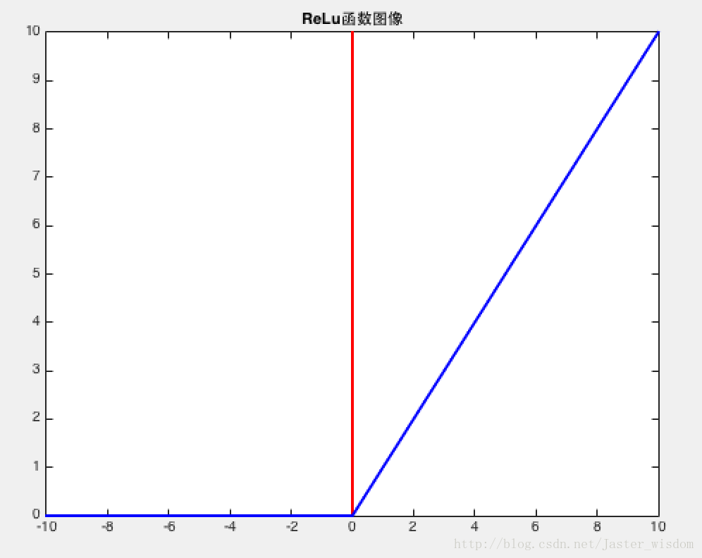
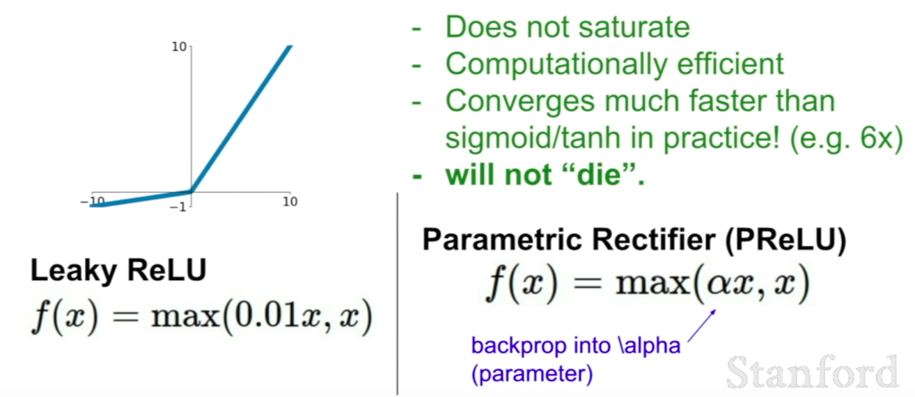
Advantages: Does not saturate (in +region); Very computationally efficient; Converges much faster than sigmoid/tanh in practice (e.g. 6x);

Disadvantages: Not zero-centered output; It kills the gradient when $x \le 0$

dead unit problem dying unit

LeakyReLu

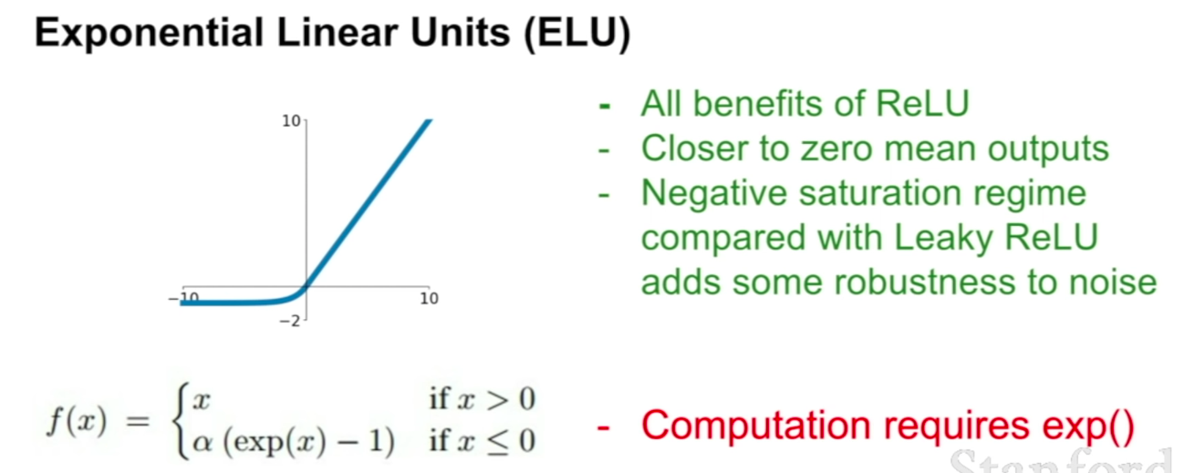
ELU

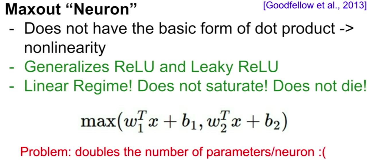
Maxout

Optimizer ref

ref

SGD

The simplest form of update is to change the parameters along the negative gradient direction (since the gradient indicates the direction of increase, but we usually wish to minimize a loss function). Assuming a vector of parameters x and the gradient dx, the simplest update has the form:

# Vanilla update
x += - learning_rate * dx

where learning_rate is a hyperparameter - a fixed constant. When evaluated on the full dataset, and when the learning rate is low enough, this is guaranteed to make non-negative progress on the loss function.

problem in sgd

Stochastic Gradient Descent with momentum

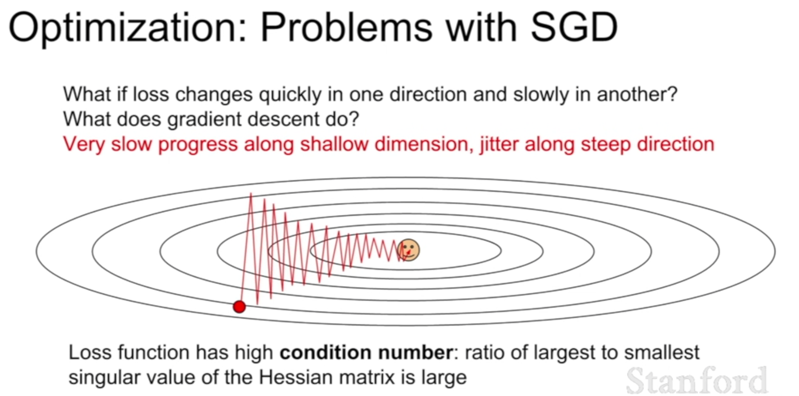
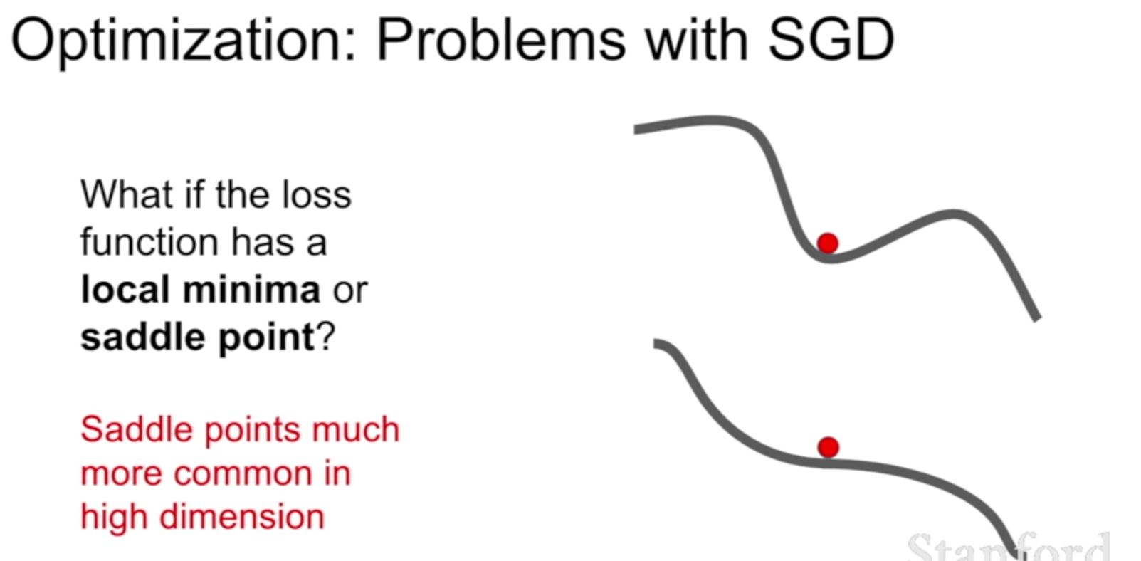
Our gradients come from minibatches so they can be noisy!

SGD+Momentum ref

Momentum is a method that helps accelerate SGD in the relevant direction and dampens oscillations.

$$v_t = \gamma v_{t-1}+\eta \Delta_{\theta}J(\theta)\\ \theta=\theta-v_t$$

The momentum term $\gamma$ tends to be 0.9/0.99.

Essentially, when using momentum, we push a ball down a hill. The ball accumulates momentum as it rolls downhill, becoming faster and faster on the way (until it reaches its terminal velocity if there is air resistance, i.e. $\gamma <1$). The same thing happens to our parameter updates: The momentum term increases for dimensions whose gradients point in the same directions and reduces updates for dimensions whose gradients change directions. As a result, we gain faster convergence and reduced oscillation.

By considering the previous gradient when computing the current gradient, there are two functions.

First of all, if the previous gradient and current gradient share the same direction, it will result in big steps to update the parameters.

Secondly, if the two gradients don’t share the same direction, we can prevent the updating step from overshooting. In other words, such low variance can help optimiization reduce the vibration on the vetical direction while moving toward to the convergence point.

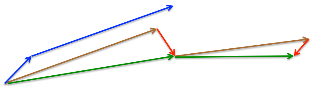
Nesterov

However, a ball that rolls down a hill, blindly following the slope, is highly unsatisfactory. We’d like to have a smarter ball, a ball that has a notion of where it is going so that it knows to slow down before the hill slopes up again.

Nesterov accelerated gradient (NAG) is a way to give our momentum term this kind of prescience. We know that we will use our momentum term $ \gamma v_{t-1}$ to move the parameters $\theta$. Computing $\theta- \gamma v_{t-1}$ thus gives us an approximation of the next position of the parameters (the gradient is missing for the full update), a rough idea where our parameters are going to be. We can now effectively look ahead by calculating the gradient not w.r.t. to our current parameters $\theta$ but w.r.t. the approximate future position of our parameters:

$$\begin{aligned} v_{t} &=\gamma v_{t-1}+\eta \nabla_{\theta} J\left(\theta-\gamma v_{t-1}\right) \\ \theta &=\theta-v_{t} \end{aligned}$$

Again, we set the momentum term $\gamma$ to a value of around 0.9. While Momentum first computes the current gradient (small blue vector in the following image) and then takes a big jump in the direction of the updated accumulated gradient (big blue vector), NAG first makes a big jump in the direction of the previous accumulated gradient (brown vector), measures the gradient and then makes a correction (red vector), which results in the complete NAG update (green vector). This anticipatory update prevents us from going too fast and results in increased responsiveness, which has significantly increased the performance of RNNs on a number of tasks.

Adagrad

Adagrad is an algorithm for gradient-based optimization that does just this: It adapts the learning rate to the parameters, performing smaller updates
(i.e. low learning rates) for parameters associated with frequently occurring features, and larger updates (i.e. high learning rates) for parameters associated with infrequent features. For this reason, it is well-suited for dealing with sparse data.

Previously, we performed an update for all parameters $\theta$ at once as every parameters $\theta_i$ used the same learning rate $\eta$. As Adagrad uses a different learning rate for every parameter $\theta_i$ at every time step $t$, we first show Adagrad’s per-parameter update, which we then vectorize. For brevity, we use $g_t$ to denote the gradient at time step $t$. $g_{t,i}$ is then the partial derivative of the objective function w.r.t. to the parameter $\theta_i$ at time step $t$:

$$g_{t, i}=\nabla_{\theta} J\left(\theta_{t, i}\right)$$

The SGD update for every parameter $\theta_i$ at each time step $t$ then becomes:

$$\theta_{t+1, i}=\theta_{t, i}-\eta \cdot g_{t, i}$$

In its update rule, Adagrad modifies the general learning rate $\eta$ at each time step $t$ for every parameter $\theta_i$ based on the past gradients that have been computed for $\theta_i$:

$$\theta_{t+1, i}=\theta_{t, i}-\frac{\eta}{\sqrt{G_{t, i i}+\epsilon}} \cdot g_{t, i}$$

$G_{t} \in \mathbb{R}^{d \times d}$ here is a diagonal matrix where each diagonal element $[i,i]$ is the sum of the squares of the gradients w.r.t. $\theta_i$ up to time step $t$, while $\epsilon$ is a smoothing term that avoids division by zero (usually on the order of $1e^{-8}$).

As $G_t$ contains the sum of the squares of the past gradients w.r.t. to all parameters $\theta$ along its diagonal, we can now vectorize our implementation by performing a matrix-vector product $\oplus$ between $G_t$ and $g_t$:

$$\theta_{t+1}=\theta_{t}-\frac{\eta}{\sqrt{G_{t}+\epsilon}} \odot g_{t}$$

Adagrad’s main weakness is its accumulation of the squared gradients in the denominator: Since every added term is positive, the accumulated sum keeps growing during training. This in turn causes the learning rate to shrink and eventually become infinitesimally small, at which point the algorithm is no longer able to acquire additional knowledge. The following algorithms aim to resolve this flaw.

RMSprop

RMSprop is an extension of Adagrad that seeks to reduce its aggressive, monotonically decreasing learning rate.

Instead of inefficiently storing $w$ previous squared gradients, the sum of gradients is recursively defined as a decaying average of all past squared gradients. The running average $E[g^2]_t$ at time step $t$ then depends (as a fraction $\gamma$ similarly to the Momentum term) only on the previous average and the current gradient:

$$E\left[g^{2}\right]_{t}=\gamma E\left[g^{2}\right]_{t-1}+(1-\gamma) g_{t}^{2} \\ \theta_{t+1}=\theta_{t}-\frac{\eta}{\sqrt{E\left[g^{2}\right]_{t}+\epsilon}} g_{t}$$

RMSprop as well divides the learning rate by an exponentially decaying average of squared gradients. Hinton suggests $\gamma$ to be set to 0.9, while a good default value for the learning rate is 0.001.

def rmsprop(w, dw, config=None):  
    """
    Uses the RMSProp update rule, which uses a moving average of squared
    gradient values to set adaptive per-parameter learning rates.

    config format:
    - learning_rate: Scalar learning rate.
    - decay_rate: Scalar between 0 and 1 giving the decay rate for the squared
      gradient cache.
    - epsilon: Small scalar used for smoothing to avoid dividing by zero.
    - cache: Moving average of second moments of gradients.
    """
    if config is None: config = {}
    config.setdefault('learning_rate', 1e-2)
    config.setdefault('decay_rate', 0.99)
    config.setdefault('epsilon', 1e-8)
    config.setdefault('cache', np.zeros_like(w))

    next_w = None
    ###########################################################################
    # TODO: Implement the RMSprop update formula, storing the next value of w #
    # in the next_w variable. Don't forget to update cache value stored in    #
    # config['cache'].                                                        #
    ###########################################################################
    # *****START OF YOUR CODE (DO NOT DELETE/MODIFY THIS LINE)*****

    next_cache = config['decay_rate'] * config['cache'] + (1 - config['decay_rate']) * dw ** 2
    next_w = w - config['learning_rate'] * dw / np.sqrt(next_cache + config['epsilon'])
    config['cache'] = next_cache

    # *****END OF YOUR CODE (DO NOT DELETE/MODIFY THIS LINE)*****
    ###########################################################################
    #                             END OF YOUR CODE                            #
    ###########################################################################

    return next_w, config

Adam

In addition to storing an exponentially decaying average of past squared gradients like RMSprop, Adam also keeps an exponentially decaying average of past gradients. Whereas momentum can be seen as a ball running down a slope, Adam behaves like a heavy ball with friction, which thus prefers flat minima in the error surface. We compute the decaying averages of past and past squared gradients $m_t$ and $v_t$ respectively as follows:

$$\begin{aligned} m_{t} &=\beta_{1} m_{t-1}+\left(1-\beta_{1}\right) g_{t} \\ v_{t} &=\beta_{2} v_{t-1}+\left(1-\beta_{2}\right) g_{t}^{2} \end{aligned}$$

$m_t$ and $v_t$ are estimates of the first moment (the mean) and the second moment (the uncentered variance) of the gradients respectively, hence the name of the method. As $m_t$ and $v_t$ are initialized as vectors of 0’s, the authors of Adam observe that they are biased towards zero, especially during the initial time steps, and especially when the decay rates are small (i.e. $\beta_1$ and $\beta_2$ are close to 1).

They counteract these biases by computing bias-corrected first and second moment estimates:

$$\begin{aligned} \hat{m}_{t} &=\frac{m_{t}}{1-\beta_{1}^{t}} \\ \hat{v}_{t} &=\frac{v_{t}}{1-\beta_{2}^{t}} \end{aligned}$$

Note that $t$ is the iteration number.

They then use these to update the parameters, which yields the Adam update rule:

$$\theta_{t+1}=\theta_{t}-\frac{\eta}{\sqrt{\hat{v}_{t}}+\epsilon} \hat{m}_{t}$$

The authors propose default values of 0.9 for $\beta_1$, 0.999 for $\beta_2$ and $10^{-8}$ for $\epsilon$.

It is worth noting that the next new m should be mt instead of $\hat m_t$.

Since Adam divide the update by $\sqrt v$, the smallest average gradients will get the larger updates. We can view the coeeficient $\frac{\eta}{\sqrt{\hat{v}_{t}}+\epsilon}$ of $\hat m_t$ as controlling, where for all gradients they share the same learning rate $ \eta $ but greater gradients have smaller $\frac{\eta}{\sqrt{\hat{v}_{t}}+\epsilon}$, which means compared to parameters with smaller gradient, the parameters with bigger gradients have samll updates.

The parameters with small gradients are in the plateau area of the cost function, and thus the moving process is slow and the training process will be slow. If we could make those parameters in plateau area get larger updates, it will help them move out of plateau quickly.

def adam(w, dw, config=None):
    """
    Uses the Adam update rule, which incorporates moving averages of both the
    gradient and its square and a bias correction term.

    config format:
    - learning_rate: Scalar learning rate.
    - beta1: Decay rate for moving average of first moment of gradient.
    - beta2: Decay rate for moving average of second moment of gradient.
    - epsilon: Small scalar used for smoothing to avoid dividing by zero.
    - m: Moving average of gradient.
    - v: Moving average of squared gradient.
    - t: Iteration number.
    """
    if config is None: config = {}
    config.setdefault('learning_rate', 1e-3)
    config.setdefault('beta1', 0.9)
    config.setdefault('beta2', 0.999)
    config.setdefault('epsilon', 1e-8)
    config.setdefault('m', np.zeros_like(w))
    config.setdefault('v', np.zeros_like(w))
    config.setdefault('t', 0)

    next_w = None
    ###########################################################################
    # TODO: Implement the Adam update formula, storing the next value of w in #
    # the next_w variable. Don't forget to update the m, v, and t variables   #
    # stored in config.                                                       #
    #                                                                         #
    # NOTE: In order to match the reference output, please modify t _before_  #
    # using it in any calculations.                                           #
    ###########################################################################
    # *****START OF YOUR CODE (DO NOT DELETE/MODIFY THIS LINE)*****

    mt = config['beta1'] * config['m'] + (1 - config['beta1']) * dw
    vt = config['beta2'] * config['v'] + (1 - config['beta2']) * dw ** 2

    t = config['t'] + 1

    mu_mt = mt / (1 - config['beta1'] ** t)
    mu_vt = vt / (1 - config['beta2'] ** t)

    next_w = w - config['learning_rate'] * mu_mt / (np.sqrt(mu_vt) + config['epsilon'])
    config['m'] = mt
    config['v'] = vt

    # *****END OF YOUR CODE (DO NOT DELETE/MODIFY THIS LINE)*****
    ###########################################################################
    #                             END OF YOUR CODE                            #
    ###########################################################################

    return next_w, config

Dropout

ref ref2

Dropout is a regularization technique. On each iteration, we randomly shut down some neurons (units) on each layer and don’t use those neurons in both forward propagation and back-propagation. Since the units that will be dropped out on each iteration will be random, the learning algorithm will have no idea which neurons will be shut down on every iteration; therefore, force the learning algorithm to spread out the weights and not focus on some specific feattures (units). Moreover, dropout help improving generalization error by:

• Since we drop some units on each iteration, this will lead to smaller network which in turns means simpler network (regularization).
• Can be seen as an approximation to bagging techniques. Each iteration can be viewed as different model since we’re dropping randomly different units on each layer. This means that the error would be the average of errors from all different models (iterations). Therefore, averaging errors from different models especially if those errors are uncorrelated would reduce the overall errors. In the worst case where errors are perfectly correlated, averaging among all models won’t help at all; however, we know that in practice errors have some degree of uncorrelation. As result, it will always improve generalization error.

We can use different probabilities on each layer; however, the output layer would always have keep_prob = 1 and the input layer has high keep_probsuch as 0.9 or 1. If a hidden layer has keep_prob = 0.8, this means that; on each iteration, each unit has 80% probablitity of being included and 20% probability of being dropped out.

It’s easy to remember things when the network has a lot of parameters (overfit), but it’s hard to remember things when effectively the network only has so many parameters to work with. Hence, the network must learn to generalize more to get the same performance as remembering things. So, that’s why Dropout will increase the test time performance: it improves generalization and reduce the risk of overfitting. ref

Therefore, at test time we multiply by dropout probability; Or, at training time, we divide by dropout probability.

The reason why we don’t apply dropout during testing is that it will make the prediction random and the evaluation will not be accurate.

Numpy Implementation

def dropout_forward(x, dropout_param):
    """
    Performs the forward pass for (inverted) dropout.

    Inputs:
    - x: Input data, of any shape
    - dropout_param: A dictionary with the following keys:
      - p: Dropout parameter. We keep each neuron output with probability p.
      - mode: 'test' or 'train'. If the mode is train, then perform dropout;
        if the mode is test, then just return the input.
      - seed: Seed for the random number generator. Passing seed makes this
        function deterministic, which is needed for gradient checking but not
        in real networks.

    Outputs:
    - out: Array of the same shape as x.
    - cache: tuple (dropout_param, mask). In training mode, mask is the dropout
      mask that was used to multiply the input; in test mode, mask is None.

    NOTE: Please implement **inverted** dropout, not the vanilla version of dropout.
    See http://cs231n.github.io/neural-networks-2/#reg for more details.

    NOTE 2: Keep in mind that p is the probability of **keep** a neuron
    output; this might be contrary to some sources, where it is referred to
    as the probability of dropping a neuron output.
    """
    p, mode = dropout_param['p'], dropout_param['mode']
    if 'seed' in dropout_param:
        np.random.seed(dropout_param['seed'])

    mask = None
    out = None

    if mode == 'train':
        #######################################################################
        # TODO: Implement training phase forward pass for inverted dropout.   #
        # Store the dropout mask in the mask variable.                        #
        #######################################################################
        # *****START OF YOUR CODE (DO NOT DELETE/MODIFY THIS LINE)*****

        mask = np.random.rand(*x.shape)>p #unpack your shape tuple using * 
        out = x*mask/p

        # *****END OF YOUR CODE (DO NOT DELETE/MODIFY THIS LINE)*****
        #######################################################################
        #                           END OF YOUR CODE                          #
        #######################################################################
    elif mode == 'test':
        #######################################################################
        # TODO: Implement the test phase forward pass for inverted dropout.   #
        #######################################################################
        # *****START OF YOUR CODE (DO NOT DELETE/MODIFY THIS LINE)*****

        out = x

        # *****END OF YOUR CODE (DO NOT DELETE/MODIFY THIS LINE)*****
        #######################################################################
        #                            END OF YOUR CODE                         #
        #######################################################################

    cache = (dropout_param, mask)
    out = out.astype(x.dtype, copy=False)

    return out, cache


def dropout_backward(dout, cache):
    """
    Perform the backward pass for (inverted) dropout.

    Inputs:
    - dout: Upstream derivatives, of any shape
    - cache: (dropout_param, mask) from dropout_forward.
    """
    dropout_param, mask = cache
    mode = dropout_param['mode']

    dx = None
    if mode == 'train':
        #######################################################################
        # TODO: Implement training phase backward pass for inverted dropout   #
        #######################################################################
        # *****START OF YOUR CODE (DO NOT DELETE/MODIFY THIS LINE)*****

        dx = mask*dout/dropout_param['p']

        # *****END OF YOUR CODE (DO NOT DELETE/MODIFY THIS LINE)*****
        #######################################################################
        #                          END OF YOUR CODE                           #
        #######################################################################
    elif mode == 'test':
        dx = dout
    return dx

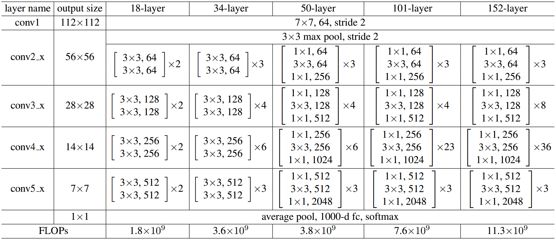
Residual Network

paper1 paper2

Motivation

simplely stack layers exhibit higher training error when the depth increases.

Models

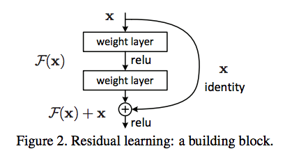
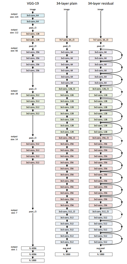
Figure from ref

pic

PatchGan

# Calculate output shape of D (PatchGAN)
patch = int(self.img_rows / 2**4)
self.disc_patch = (patch, patch, 1)

# Build and compile the discriminator
self.discriminator = self.build_discriminator()
self.discriminator.compile(loss='mse',optimizer=optimizer,metrics=['accuracy'])

def build_discriminator(self):
    def d_layer(layer_input, filters, f_size=4, bn=True):
        d = Conv2D(filters, kernel_size=f_size, strides=2, padding='same')(layer_input)
        d = LeakyReLU(alpha=0.2)(d)
        if bn:
            d = BatchNormalization(momentum=0.8)(d)
        return d
    img_A = Input(shape=self.img_shape)
    img_B = Input(shape=self.img_shape)
    combined_imgs = Concatenate(axis=-1)([img_A, img_B])
    d1 = d_layer(combined_imgs, self.df, bn=False)
    d2 = d_layer(d1, self.df*2)
    d3 = d_layer(d2, self.df*4)
    d4 = d_layer(d3, self.df*8)
    validity = Conv2D(1, kernel_size=4, strides=1, padding='same')(d4)
    return Model([img_A, img_B], validity)
def train(self):
    valid = np.ones((batch_size,) + self.disc_patch)
    fake = np.zeros((batch_size,) + self.disc_patch)
    
    for epoch in range(epochs):
        fake_A = self.generator.predict(imgs_B)
        d_loss_real = self.discriminator.train_on_batch([imgs_A, imgs_B], valid)
        d_loss_real = self.discriminator.train_on_batch([imgs_A, imgs_B], valid)
        d_loss = 0.5 * np.add(d_loss_real, d_loss_fake)
        
        g_loss = self.combined.train_on_batch([imgs_A, imgs_B], [valid, imgs_A])

• The output of discriminator is (None, patch, patch, 1), which can be seen using model.summary(). While the traditional discriminator’s output is (None, 1), distinguishing each image.

• If traditional discriminator, the last two line codes would be:

  >   d5 = Flatten()(d4)
  >   validity = layers.Dense(1,activation='sigmoid')(d5)
  >   return Model([img_A, img_B], validity)
  >

>

​