Logistic Regression

用于分类任务的逻辑斯蒂回归。

逻辑斯蒂回归

模型

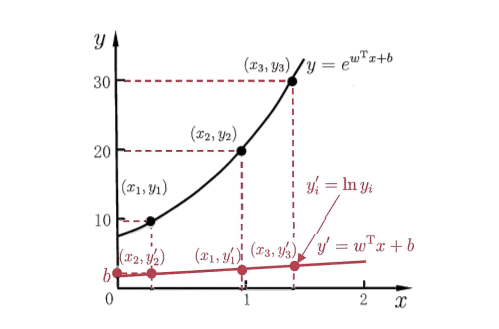
线性回归试图用一个线性函数的预测值取逼近真实值，那么是否能用一个线性函数的预测值去逼近真实值的衍生值呢？假设我们使用预测值去逼近一个对数函数$g(y)=In(y)$，那么$g(y)=f(y)$，

$$In(y)=w^Tx+b$$

这样我们就得到了对数线性回归，它实际上是试图让$e^{(w^Tx+b)}$去逼近$y$，本质上仍然是线性回归，但已是在求输入空间到输出空间的非线性函数的映射。如下图所示，指数空间的真实值通过对数函数映射到一个线性空间：

线性模型可以用于回归学习，但是如果要做的是分类任务该如何？启发自对数线性回归，我们可以找到一个类似对数函数的一个单调可微函数将分类任务的真实标记$y$映射到线性回归模型的预测值。

考虑二分类问题，其输出标记是$y\in\{0,1\}$，而线性回归模型的预测值$z=w^Tx+b$是实值，故使用一个阶跃函数，进行实值与离散值的映射：

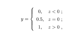
若预测值$z$大于零就判为正例，小于零就判为负例，预测值为临界值零则任意判断，

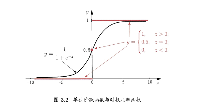
因为阶跃函数是不连续的，所以我们使用了一个连续可微的函数替代函数：

$$y=\frac{1}{1+e^{-z}}=\frac{1}{1+e^{-(w^Tx+b)}}$$

上式可变化为：

$$In\frac{y}{1-y}=w^Tx+b$$

如果将$y$看作样本$x$作为正例的概率，则$1-y$表示反例的概率，两者的比值反映了$x$作为正例的相对可能性，称为几率，对几率取对数称为对数几率。可以看出上式用线性回归模型的预测值去逼近真实标记的对数几率，因为对应模型称为逻辑斯蒂回归。需要注意的是虽然名字是”回归”，但是它是分类方法。

算法求解

如果将预测值$y$看作类后验概率估计$p(y=1|x)$，则上式：

$$In(\frac{p(y=1|x)}{p(y=0|x)})=w^Tx+b$$

又因为$p(y=1|x)+p(y=0|x)=1$，所以联合求解得到：

$$p(y=1|x)=\frac{e^{w^Tx+b}}{1+e^{w^Tx+b}}\\ p(y=1|x)=\frac{1}{1+e^{w^Tx+b}}$$

可以通过极大似然法求解：

$$max \ P=\prod_{i=1}^{m}[p(y=1|x_i)^{y_i}p(y=0|x_i)^{(1-y_i)}]$$

即令每个样本属于其真实标记的概率越大越好，两边取对数：

$$max\ In(P)=\sum_{i=1}^{m}y_iIn[p(y=1|x_i)]+(1-y_i)In[p(y=0|x_i)]$$

如果真实标记$y_i=1$，则$y_iIn[p(y=1|x_i)]+(1-y_i)In[p(y=0|x_i)]=p(y=1|x_i)$；

如果真实标记$y_i=0$，则$y_iIn[p(y=1|x_i)]+(1-y_i)In[p(y=0|x_i)]=p(y=0|x_i)$；

即：

$$max \ In(Loss)=\sum_{i=1}^{m}y_i(w^Tx+b)+In(\frac{1}{e^{w^Tx+b}+1})$$

max上式等价于：

$$min \ In(Loss)=\sum_{i=1}^{m}-y_i(w^Tx+b)+In({1+e^{w^Tx+b}})$$

可以使用梯度下降法求解最佳的$w$和$b$：

$$w_j=w_j-\alpha\sum_{i=1}^{n}(h_w(x^{(i)})-y^{(i)})x_{j}^{(i)}$$

样本集$D\{(x_i,y_i)\}^{n}_{i=1}$, 利用最大似然法, 即令每个样本属于其真实标签的概率越大越好，故似然函数为

$$\prod_{i=1}^{n}p^{y_i}(1-p)^{(1-y_i)}$$

对数似然函数:

$$L(p)=\sum_{i=1}^{n}y_iInP+\sum_{i=1}^{n}(1-y_i)In(1-p)$$

对$P$求$w$导数:

$$P=\frac{1}{1+e^{-(wx+b)}}\\ \frac{\partial{P}}{\partial{w}}=\frac{-1}{(1+e^{-(wx+b)})^2}*e^{-(wx+b)}*-x=P(1-P)$$

$L(P)$对$w$求导数:

$$\frac{\partial{L(P)}}{\partial{w}}=\sum_{i=1}^{n}y_i\frac{1}{P}\frac{\partial{P}}{\partial{w}}+\sum_{i=1}^{n}(1-y_i)\frac{-1}{1-p}\frac{\partial{P}}{\partial{w}}=XY(1-P)+(-1+Y)XP=(Y-P)X$$

正则化

目标函数

$$E(w,b)=-\frac{1}{n}[\sum_{i=1}^{n}y^{(i)}logh_w(x^{(i)})+(1-y^{(i)})log(1-h_w(x^{(i)}))]+\lambda\sum_{i=1}^{n}w_{i}^{2}$$

梯度下降法

$w_0=w_0-\alpha\frac{1}{n}\sum_{i=1}^{n}(h_w(x^{(i)})-y^{(i)})x_0^{(i)}$

$w_j=w_j-\alpha[\frac{1}{n}\sum_{i=1}^{n}(h_w(x^{(i)})-y^{(i)})x_j^{(i)}-\frac{\lambda}{n}w_j]$

Softmax Loss - Multinomial Logistic Regression

对于多分类任务，模型的输出是一个多维向量，向量的每一位表示该输出属于某一类的概率。softmax则将输出建模成一个分布：

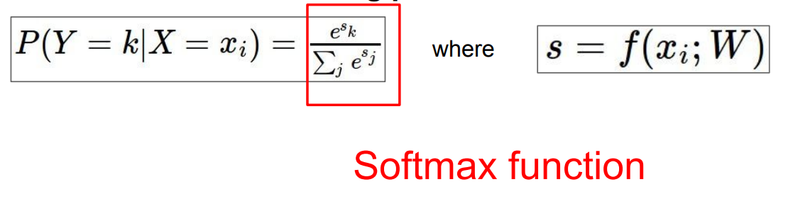
其中，$x_i$是第$i$个输入，$k$表示某一个类，则上式计算该输入属于某一个类的概率。

那么我们的损失函数就变成了：

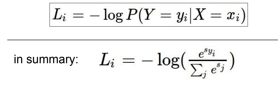
对于每一个样本，我们最大化它属于正确类的概率。因为$ 0\le P(Y=y_i|X=x_i)\le 1$,所以$logP<0$；我们追求的是$P()$越大，$L_i$越小，但是对于$logP$, 恰恰相反，所以对损失函数取负。

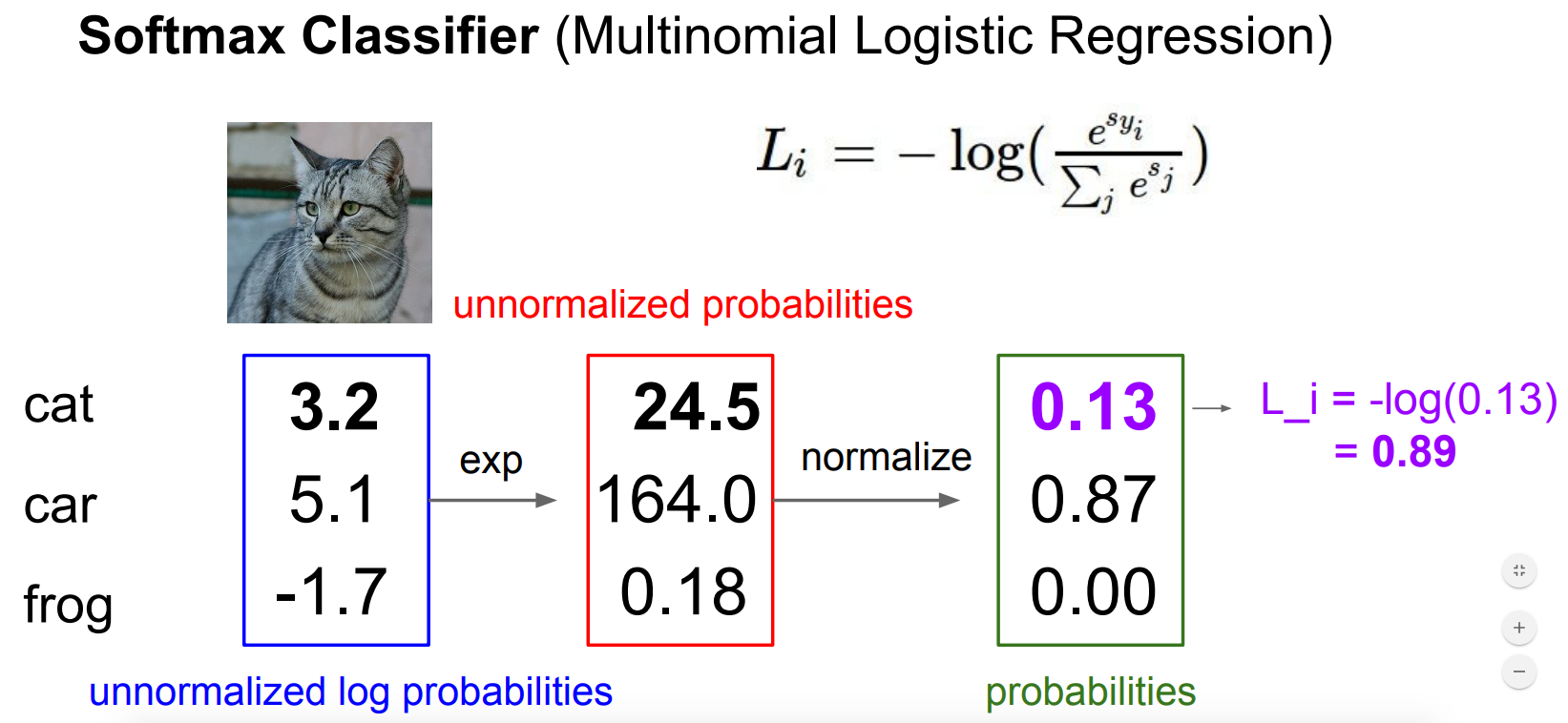
对于上面的例子，分类器的输出是$(3.2,5.1,-1.7)$,经过softmax函数计算，我们得到$(0.13,0.87,0.0)$，那么该样本的损失为$L_i=-log(0.13)$.

1. What is the min/max possible loss $L_i$?

   The min loss is 0 when we classify the input correctly with a extremely high score. The max loss is $\infin$ when we classify the input to the correct category with a extremely low score. And according to the figure, it is infinite.

2. Usually at initialization $W$ is small so all $s\approx 0$. What is the loss?

   The answer is $-log(\frac{1}{C})$, where $C$ is the class number.

Softmax Forward

ref1 ref2

Softmax function takes an N-dimensional vector of real number and transforms it into a vector of real number in range $(0,1)$ which add up to 1. For each output element $a_j$ in the last layer:

$$f(a_j)=\frac{e^{a_j}}{\sum_{i=1}^{k}e^{a_i}}$$

In python, we have the code for softmax function as follows:

def softmax(x):
    exps = np.exp(x)
    return exps/np.sum(exps)

We have to note that the numerical range of float number in numpy is limited. For float64 the upper bound is $10^{308}$. For exponential, it is not difficult to overshoot that limit, in which case python returns nan.

To make our softmax function numerically stable, we simply normalize the values in the vector, by multiplying the numerator and denominator with a constant $C$.

$$\begin{align} p_i &= \frac{e^{a_i}}{\sum_{k=1}^N e^{a_k}} \\ &= \frac{Ce^{a_i}}{C\sum_{k=1}^N e^{a_k}} \\ &= \frac{e^{a_i + \log(C)}}{\sum_{k=1}^N e^{a_k + \log(C)}} \\ \end{align}$$

We can choose an arbitrary value for $log(C)$ term, but generally $log(C)=−max(a)$ is chosen, as it shifts all of elements in the vector to negative to zero, and negatives with large exponents saturate to zero rather than the infinity, avoiding overflowing and resulting in nan.

The code for our stable softmax is as follows:

def softmax(x):
    exps = np.exp(x-np.max(x))
    return exps/np.sum(exps)

Derivative

Due to the desirable property of softmax function outputting a probability distribution, we use it as the final layer in neural networks. For this we need to calculate the derivative or gradient and pass it back to the previous layer during backpropagation.

For each node $a_j$ in the output layer, we want to calculate:

$$\frac{\partial p_i}{\partial a_j} = \frac{\partial \frac{e^{a_i}}{\sum_{k=1}^N e^{a_k}}}{\partial a_j}$$

If $i=j$:

$$\begin{align} \frac{\partial \frac{e^{a_i}}{\sum_{k=1}^N e^{a_k}}}{\partial a_j}&= \frac{e^{a_i} \sum_{k=1}^N e^{a_k} - e^{a_j}e^{a_i}}{\left( \sum_{k=1}^N e^{a_k}\right)^2} \\ &= \frac{e^{a_i} \left( \sum_{k=1}^N e^{a_k} - e^{a_j}\right )}{\left( \sum_{k=1}^N e^{a_k}\right)^2} \\ &= \frac{ e^{a_j} }{\sum_{k=1}^N e^{a_k} } \times \frac{\left( \sum_{k=1}^N e^{a_k} - e^{a_j}\right ) }{\sum_{k=1}^N e^{a_k} } \\ &= p_i(1-p_j) \end{align}$$

For $i\ne j$:

$$\begin{align} \frac{\partial \frac{e^{a_i}}{\sum_{k=1}^N e^{a_k}}}{\partial a_j}&= \frac{0 - e^{a_j}e^{a_i}}{\left( \sum_{k=1}^N e^{a_k}\right)^2} \\ &= \frac{- e^{a_j} }{\sum_{k=1}^N e^{a_k} } \times \frac{e^{a_i} }{\sum_{k=1}^N e^{a_k} } \\ &= - p_j.p_i \end{align}$$

So the derivative of the softmax function is given as,

$$\frac{\partial p_i}{\partial a_j} = \begin{cases}p_i(1-p_j) & if & i=j \\ -p_j.p_i & if & i \neq j \end{cases}$$

Or using Kronecker delta $\delta{ij} = \begin{cases} 1 & if & i=j \\ 0 & if & i\neq j \end{cases}$

$$\frac{\partial p_i}{\partial a_j} = p_i(\delta_{ij}-p_j)$$

Cross Entropy Loss

Corss entropy loss indicates the distance between what the model belives the output distribution should be, and what the original distribution really is. It is defined as:

$$H(y,p) = - \sum_i y_i log(p_i)$$

It is widely used as an alternative of squared error. It is used when node activations can be understand as representing the probability that each hypothesis might be true, i.e. when the output is a probability is a probability distribution. Thus it is used as a loss function in neural networks which have softmax activations in the output layer:

def cross_entropy(x,y):
    """
    X is the output from fully connected layer (num_examples x num_classes)
    y is labels (num_examples x 1)
    	Note that y is not one-hot encoded vector. 
    	It can be computed as y.argmax(axis=1) from one-hot encoded vectors of labels if required.
    """
    l = y.shape[0]
    prob = softmax(x)
    prob_of_groundtruth = [row[y[i]] for i,row in enumerate(prob)]
    log_likelihood = -np.log(prob_of_groundtruth)
    loss = np.sum(log_likelihood)
    return loss

Derivative of Cross Entropy Loss with Softmax

Cross Entropy Loss with Softmax function are used as the output layer extensively. Now we use the derivative of softmax that we derived earlier to derive the derivative of the cross entropy loss function.

For each sample $(x_i,y_i)$, there are $c$ classes

$$\begin{align} L_i &= - \sum_i^c y_i log(p_i) \\ \end{align}$$

Then for each output node $o_i$, i.e., score of the class $i$ :

$$\begin{align} \frac{\partial L_i}{\partial o_i} &= - \sum_k y_k \frac{\partial log(p_k)}{\partial o_i } \\ &= - \sum_k y_k \frac{\partial log(p_k)}{\partial p_k} \times \frac{\partial p_k}{ \partial o_i} \\ &= - \sum y_k \frac{1}{p_k} \times \frac{\partial p_k}{\partial o_i} \\ \end{align}$$

From derivative of softmax we derived earlier that $\frac{\partial p_i}{\partial a_j} = \begin{cases}p_i(1-p_j)& if & i=j \\ -p_j.p_i & if & i \neq j\end{cases}$,

$$\begin{align} \frac{\partial L}{\partial o_i} &= -y_i(1-p_i) - \sum_{k\neq i} y_k \frac{1}{p_k}(-p_k.p_i) \\ &= -y_i(1-p_i) + \sum_{k \neq 1} y_k.p_i \\ &= - y_i + y_ip_i + \sum_{k \neq 1} y_k.p_i \\ &= p_i\left( y_i + \sum_{k \neq 1} y_k\right) - y_i \\ &= p_i\left( y_i + \sum_{k \neq 1} y_k\right) - y_i \end{align}$$

$y$ is a one hot encoded vector for the label, so $\sum_{k}y_k =1$, and $y_i + \sum_{k\ne i}y_k =1$. So we have,

$$\frac{\partial L}{\partial o_i} = p_i - y_i$$

def delta_cross_entropy(x,y):
    """
    X is the output from fully connected layer (num_examples x num_classes)
    y is labels (num_examples x 1)
    	Note that y is not one-hot encoded vector. 
    	It can be computed as y.argmax(axis=1) from one-hot encoded vectors of labels if required.
    """
    m = y.shape[0]
    prob = softmax(x)
    prob_of_groundtruth = [row[y[i]] for i,row in enumerate(prob)]
    prob_of_groundtruth -= 1
    return prob_of_groundtruth/m

In summary, the overall loss of cross entropy loss with sigmoid function is as following:

for each sample $(x_i,y_i)$,

$$Loss=-\frac{1}{n}\sum_{i}^{n}y_ilog(p_i) + \frac{1}{2}\sum_{m}\sum_{n}w_{m,n}^{2}\\ p_i=\frac{e^{o_i}}{\sum_{k}^{c}e^{o_k}}$$

where $o_i$ is the non-logit output, $p_i$ is the probability of being class $i$, $y_i$ is the groundtruth class. The second part of $Loss$ is the regularization.

Numpy Implementation

The plaint implementation is as following:

import numpy as np

class Softmax():
    def __init__(self):
        self.W = None
    def softmax_loss_naive(self,W, X, y, reg):
        '''
        :param W:A numpy array of shape (D, C) containing weights.
        :param X:A numpy array of shape (N, D) containing a minibatch of data.
        :param y:A numpy array of shape (N,) containing training labels; y[i] = c means
        that X[i] has label c, where 0 <= c < C.
        :param reg:(float) regularization strength
        :return:a tuple of:
                 - loss as single float
                 - gradient with respect to weights W; an array of same shape as W
        '''
        loss = 0.0
        dW = np.zeros_like(W)
        D, C = W.shape
        N, D = X.shape
        scores = X.dot(W)
        norm_scores = scores - np.max(scores, axis=1).reshape(-1, 1)
        prob_scores = np.exp(norm_scores)
        prob_scores /= np.sum(prob_scores, axis=1).reshape(-1, 1)
        for i in range(N):
            loss -= np.log(prob_scores[i][y[i]])
        loss = loss / N + reg * 0.5 * np.sum(W ** 2)

        for i in range(N):
            for c in range(C):
                if y[i] == c:
                    dW[:, c] += X[i] * (prob_scores[i][c] - 1)
                else:
                    dW[:, c] += X[i] * prob_scores[i][c]
        dW = dW / N + reg * W
        return loss, dW

    def softmax_loss_vectorized(self,W, X, y, reg):

        loss = 0.0
        dW = np.zeros(W.shape)

        D, C = W.shape
        N, D = X.shape
        scores = X.dot(W)
        norm_scores = scores - np.max(scores, axis=1).reshape(-1, 1)
        prob_scores = np.exp(norm_scores)
        prob_scores /= np.sum(prob_scores, axis=1).reshape(-1, 1)

        # LOSS Calculation
        loss = -1 * np.sum(np.log(prob_scores[np.arange(N), y]))
        loss = loss / N + reg * 0.5 * np.sum(W ** 2)

        # Gradient Calculation
        prob_scores[np.arange(N), y] -= 1
        dW = X.T.dot(prob_scores)
        dW = dW / N + reg * W

        return loss, dW

    def loss(self, X_batch, y_batch, reg):
        return self.softmax_loss_vectorized(self.W, X_batch, y_batch, reg)

    def train(self, X, y, learning_rate=1e-3, reg=1e-5, num_iters=100,
              batch_size=200, verbose=False):
        '''

        :param X:A numpy array of shape (N, D) containing training data; there are N
          training samples each of dimension D.
        :param y:A numpy array of shape (N,) containing training labels; y[i] = c
          means that X[i] has label 0 <= c < C for C classes.
        :param learning_rate:(float) learning rate for optimization.
        :param reg:(float) regularization strength.
        :param num_iters:(integer) number of steps to take when optimizing
        :param batch_size:(integer) number of training examples to use at each step.
        :param verbose:(boolean) If true, print progress during optimization.
        :return:A list containing the value of the loss function at each training iteration.
        '''
        num_train, dim = X.shape
        num_classes = np.max(y) + 1  # assume y takes values 0...K-1 where K is number of classes
        if self.W is None:
            # lazily initialize W
            self.W = 0.001 * np.random.randn(dim, num_classes)

        # Run stochastic gradient descent to optimize W
        loss_history = []
        for it in range(num_iters):
            mask = np.random.choice(num_train, batch_size)
            X_batch = X[mask]
            y_batch = y[mask]

            # evaluate loss and gradient
            loss, grad = self.loss(X_batch, y_batch, reg)
            loss_history.append(loss)
            self.W -= learning_rate * grad
            if verbose and it % 100 == 0:
                print('iteration %d / %d: loss %f' % (it, num_iters, loss))
        return loss_history

    def predict(self, X):
        scores = X.dot(self.W)
        y_pred = np.argmax(scores,axis=1)
        return y_pred

多分类学习

目前我们接触的问题是二分类问题，即每一个样本的label只有两种可能性(0|1)。但是，有时候会碰到多分类问题，即每一个样本label有两种以上的选择，比如对水果图片进行分类的任务就是多分类任务，因为一张图片可能是苹果，香蕉，橘子或者草莓等。

多分类的学习思路是将多分类任务拆分成若干个二分类任务求解，经典的拆分方法有三种：“一对一”(One vs One，简称OvO)，“一对余”(One vs Rest，简称OvR)和“多对多”(Many vs Many，简称MvM)。

一对一（OvO）

思想：给定具有$N$个类别的数据集，分为$N$个类别的堆，两两一组，一正一反，训练出$\frac{N(N-1)}{2}$个分类器。测试的时候，将测试样本送给所有的分类器，故产生$\frac{N(N-1)}{2}$个结果，投票选出最终的类别。

from sklearn import datasets
from sklearn.multiclass import OneVsOneClassifier
from sklearn.svm import LinearSVC

iris = datasets.load_iris()
x,y = iris.data, iris.target
model = OneVsOneClassifier(LinearSVC(random_state=0))
model.fit(x,y)
re = model.predict(x)
print(re)

一对余(OvR)

思想：每次将一个类的样例作为正类，剩下的其他类的样例作为反例来训练$N$个分类器。测试时，若仅有一个分类器预测为正类，则对应的类别作为最终的分类结果。若有多个分类器预测为正类，则通常考虑各分类器的预测置信度，选择置信度最大的类别标记为分类结果。

from sklearn import datasets
from sklearn.multiclass import OneVsRestClassifier
from sklearn.svm import LinearSVC
iris = datasets.load_iris()
X, y = iris.data, iris.target
OneVsRestClassifier(LinearSVC(random_state=0)).fit(X, y).predict(X)

比较：

类别不平衡

ref1

定义

机器学习中常常会遇到数据的类别不平衡（class imbalance），也叫数据偏斜（class skew）。以常见的二分类问题为例，我们希望预测病人是否得了某种罕见疾病。但在历史数据中，阳性的比例可能很低（如百分之0.1）。在这种情况下，学习出好的分类器是很难的，而且在这种情况下得到结论往往也是很具迷惑性的。

以上面提到的场景来说，如果我们的分类器总是预测一个人未患病，即预测为反例，那么我们依然有高达99.9%的预测准确率。然而这种结果是没有意义的。

解决方法

• 试用其他评价指标
• 对数据集进行重采样
• ​

例子

需要一个标准对数据进行约束：

1. x增加全1行

2. shape

   x.shape = (m,n) # m:样本数；n：特征数
   y.shape = (m,) # 一维行向量
   thetas = (n,1) # 一维列向量

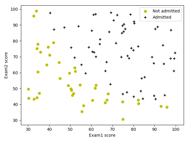
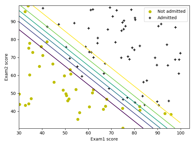
预测是否录取学生 ref

数据集包含学生的两次考试成绩以及其是否被录取的信息。

数据加载

数据载入的方式千千万万种方式，但是一旦载入之后，需要做的操作包括：

data = np.loadtxt('./dataset/ex2data1.txt',delimiter=',')
x = np.array(data[:,:-1])
y = np.array(data[:,-1])

row,_ = np.shape(x)
ones = np.ones((row,1))
x_new = np.concatenate((ones,x),axis=1)
_,col = np.shape(x_new)
thetas = np.zeros([col,1])

数据可视化

def plot_data(x,y):
    plt.scatter(x[y==0,0],x[y==0,1],marker='o',label='Not admitted',c = 'y')
    plt.scatter(x[y == 1, 0], x[y == 1, 1], marker='+', label='Admitted',c='black')
    plt.xlabel('Exam1 score')
    plt.ylabel('Exam2 score')
    plt.legend()

Sigmoid激活函数

我们的sigmoid函数为：

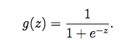
在实现激活函数之后，我们使用几个值取测试是否写对了：如果激活函数的输入是很大的值，那么我们的输出应该接近1；如果是很小的数，应该接近0；如果输入0，则输出0.5。而且，输入不应区分向量，矩阵的。

def sigmoid(z):
    gz = 1 / (1 + np.exp(-z))
    return gz

代价函数和梯度下降法

def cost_func(thetas,x,y):
    z = x.dot(thetas)
    y_pred = sigmoid(z)
    loss = y.T.dot(np.log(y_pred)) + (1-y).T.dot(np.log(1-y_pred))
    return -loss/row

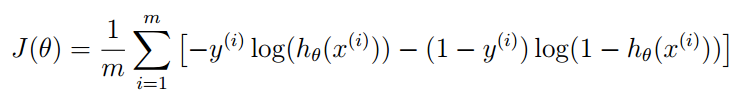
初次调用时，loss=0.693

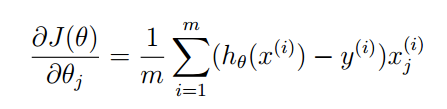
这次我们的梯度下降法返回梯度量，不直接返回参数更新

def gradient_descent(thetas,x,y):
    z = x.dot(thetas)
    y_pred = sigmoid(z)
    gd = (y_pred-y).T.dot(x) / row
    return gd.T

损失函数优化

这次，我们使用scipy.optimize寻找目标函数的最优值。

scipy.optimize.fmin_tnc(func, x0, fprime=None, args=())

• func：目标函数，它必须满足以下条件之一：

  — 返回函数值f和梯度值g

  — 返回函数值f，但是必须提供梯度函数作为fprime的参数

  —返回函数值f，设置 approx_grad=True

• x0：待优化参数的初始值

• fprime：梯度函数

• args：func函数的参数

• 该函数的返回值：x—solution；nfeval—函数优化次数；

最优化之后的损失函数值是0.203左右。

import scipy.optimize as opt
def scipy_gd(thetas,x,y):
    result = opt.fmin_tnc(
        func=cost_func,x0=thetas,fprime=gradient_descent,args=(x,y))
    return result[0]

预测及评价

我们定义一个预测函数，输入未知值，预测其分类

def predict(thetas,x):
    z = x.dot(thetas)
    prob = sigmoid(z)
    return [1 if x >= 0.5 else 0 for x in prob]

使用准确率来评估预测结果

if __name__ == '__main__':
    thetas = scipy_gd(thetas,x_new,y)
    predictions = predict(thetas,x_new)
    correct = [1 if ((a == 1 and b == 1) or (a == 0 and b == 0)) else 0 for (a, b) in zip(predictions, y)]
    accuracy = (sum(map(int, correct)) % len(correct))
    plot_boundary(x,y,thetas)

画出分类边界

需要注意的是，此时的x并不需要额外的全1行。

import matplotlib.pylab as pl
def plot_boundary(x,y,thetas):
    plot_data(x,y)
    h = 0.1
    x0_min, x0_max = x[:, 0].min() - 0.1, x[:, 0].max() + 0.1
    x1_min, x1_max = x[:, 1].min() - 0.1, x[:, 1].max() + 0.1
    x0, x1 = np.meshgrid(np.arange(x0_min, x0_max, h),
                         np.arange(x1_min, x1_max, h))
    z = np.c_[x0.ravel(), x1.ravel()].dot(thetas[1:]) + thetas[0]
    z = sigmoid(z)
    z = z.reshape(x0.shape)
    plt.contour(x0, x1, z, cmap=pl.cm.Paired)
    plt.show()

正则化的回归

ref

本题我们使用正则化的逻辑斯蒂回归来分类。给定的数据集是关于微芯片的两次测试数据，label是合格与不合格。

1. 数据可视化

   直接利用上面的画图函数，可以看到我们需要使用一个非线性曲线去分类，类似椭圆。显然这不能是线性分类，对于非线性分类问题，逻辑回归会使用多项式扩展特征。这带来的弊端就是引入巨大特征。

   

2. ​

逻辑斯蒂回归预测西瓜

1. 数据载入

   import numpy as np  
   import matplotlib.pyplot as plt
   dataset = np.loadtxt('watermelon_3a.csv', delimiter=",")
   X = dataset[:, 1:3]
   y = dataset[:, 3]
   m, n = np.shape(X)

2. 数据可视化

   # draw scatter diagram to show the raw data
   f1 = plt.figure(1)
   plt.title('watermelon_3a')
   plt.xlabel('density')
   plt.ylabel('ratio_sugar')
   plt.scatter(X[y == 0, 0], X[y == 0, 1], marker='o', color='k', s=100, label='bad')
   plt.scatter(X[y == 1, 0], X[y == 1, 1], marker='o', color='g', s=100, label='good')
   plt.legend(loc='upper right')
   plt.show()

   

3. 利用sklearn求解

   from sklearn import metrics
   from sklearn import model_selection
   from sklearn.linear_model import LogisticRegression
   import matplotlib.pylab as pl
   X_train, X_test, y_train, y_test = model_selection.train_test_split(X, y, test_size=0.5, random_state=0)
   log_model = LogisticRegression()  
   log_model.fit(X_train, y_train) 
   weights , b = log_model.coef_, log_model.intercept_
   # weights = [[-0.0865987   0.39410864]] 
   # b = [-0.02152586]

4. 结果可视化

   ###计算模型各种评价标准
   print(metrics.confusion_matrix(y_test, y_pred))
   print(metrics.classification_report(y_test, y_pred))
   y_pred = log_model.predict(X_test)
   precision, recall, thresholds = metrics.precision_recall_curve(y_test, y_pred)

   h = 0.001
   x0_min, x0_max = X[:, 0].min() - 0.1, X[:, 0].max() + 0.1
   x1_min, x1_max = X[:, 1].min() - 0.1, X[:, 1].max() + 0.1
   x0, x1 = np.meshgrid(np.arange(x0_min, x0_max, h),
                        np.arange(x1_min, x1_max, h))
   z = log_model.predict(np.c_[x0.ravel(), x1.ravel()])
   z = z.reshape(x0.shape)
   plt.contourf(x0, x1, z, cmap=pl.cm.Paired)
   plt.contour(x0, x1, z, cmap=pl.cm.Paired)

   • meshgrid 通俗说，输入是两个一维向量x和y，对于y中的每一个值$y_i$，都为之复制一个x，相当于从$y_i$出发画一条平行x轴的直线，有多少个y点，就有多少条直线；同理，对于x中的灭一个$x_i$，为之复制一个y，等价于从该$x_i$出发画一条平行于$y$轴的直线。这样很多条直线相交就会产生$len(y) \ \cdot \ len(x)$形状的矩阵。
   • np.c_[a,b]将两数组在column方向合并,等价于np.concatenate((a,b),axis=1)
   • np.ravel()将数组展开，多维降为一维，类似np.flatten()，只不过np.flatten()返回拷贝，而ravel()返回视图，会对原始数组产生影响。

   

   

交叉验证法 vs 留一法

基于UCI数据集，比较10折交叉验证和留一法所估计出的对率回归的准确率。

我们选择Iris数据和blood transfusion数据

Iris数据共有4个特征个一个类别label。

第一个是sepal length，第二个是sepal width，第三个是petal length，第四个特征是petal width。类别有三类：— Iris Setosa — Iris Versicolour — Iris Virginica

blood transfusion数据总共有4个特征和一个label。

R(Recency):距离上次献血时间(month)
F(Frequency):总献血次数
M(Monetary):总献血量
T(Time):距离第一次献血(month)
Y:2007的三月是否献血;1-献血，0-没有献血

import seaborn as sns
import matplotlib.pyplot as plt
import pandas as pd

def plot_data(data,y):
    sns.set(style='white',color_codes=True)
    sns.pairplot(data,hue=y)
    plt.show()

if __name__ == '__main__':

    iris = sns.load_dataset('iris')
    plot_data(iris,'species')

    data = pd.read_csv('blood_dataset.txt',sep=',',header=None)
    data.columns = ['R','F','M','T','Y']
    plot_data(data,'Y')

from sklearn.datasets import load_iris
from sklearn.model_selection import cross_val_predict, LeaveOneOut
from sklearn.linear_model import LogisticRegression
from sklearn import metrics
import numpy as np

def cv(x,y):
    log_regression = LogisticRegression()
    pre = cross_val_predict(log_regression,x,y,cv=5)
    print(metrics.accuracy_score(y,pre))

def loo(x,y):
    loo = LeaveOneOut()
    accuracy = 0
    log_regression = LogisticRegression()
    for train,test in loo.split(x):
        log_regression.fit(x[train],y[train])
        y_p = log_regression.predict(x[test])
        if y_p == y[test] : accuracy += 1
    print(accuracy/np.shape(x)[0]) # 0.9533333333333334
def load_blood():
    data = np.loadtxt('blood_dataset.txt',delimiter=',') #shape = (748,5)
    x = data[:,:-1] # shape = (748, 4)
    y = data[:,-1] # shape = (748,)
    return x,y

if __name__ == '__main__':

    iris = load_iris()
    x = iris.data  # x.shape = (150,4)
    y = iris.target  # x.shape = (150,)
    cv(x,y) # 0.96
    loo(x,y) # 0.9533333333333334

    x,y=load_blood()
    cv(x,y) # 0.7807486631016043
    loo(x,y) # 0.7700534759358288

也可以看到，两种交叉验证的结果相近，但是由于此数据集的类分性不如iris明显，所得结果也要差一些。同时由程序运行可以看出，LOOCV的运行时间相对较长，这一点随着数据量的增大而愈发明显。

所以，一般情况下选择K-折交叉验证即可满足精度要求，同时运算量相对小。