支持向量机(SVM)是一个用于分类和回归的线性模型，它可以解决线性和非线性问题。

支持向量机的思想很简单：我们尽量找到一条直线或者一个超平面将数据集分成不同的类。

在逻辑斯蒂回归中，我们用了sigmoid激活函数将$y=wx+b$的计算结果压缩到$[0,1]$范围内，这样，如果我们的压缩值大于临界值0.5，我们就将该样例分类到正例；否则我们将之分类到负例。在SVM中，我们将临界值设置为-1和+1，即如果$y=wx+b$的计算结果大于1，我们分类至正例；如果$y=wx+b$的计算结果小于-1，我们分类至负例，这样我们就得到了一个区间$[-1,1]$，称之为间隔。

Introduction

给定数据集$D=\{(x_1,y_1), (x_2,y_2),…,(x_m,y_m)\}, y_i\in{\{-1,+1\}}$, 欲找到一个划分超平面, 将不同类别的样本分开.

1_VDATmWG1E1ZNg7hdasOh5g

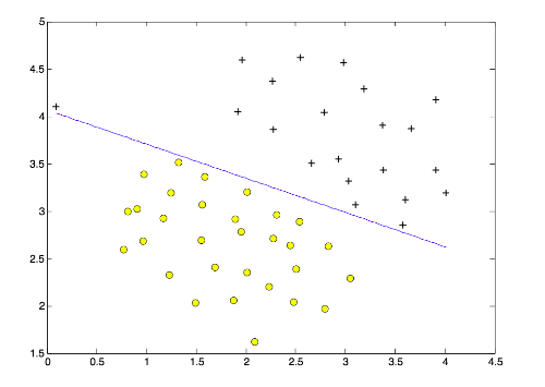
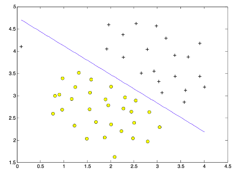
但是能将训练样本分开的划分超平面有多个, 直观上, 去找位于两类样本”正中间”的划分超平面, 即下图中的黄线是比较好的分割线。可用线性方程描述:

$w^Tx+b=0$

1_AMR3v-jCvUMXPUtQskzxmQ

那么如何用数学方法描述黄色的那条直线是比较好的分割线呢？使用点到直线的距离，我们欲使直线两边的点离直线的距离越远越好，这样不同类的点也距离越远，说明我们的分割线比较明确地分类出正类和负类。

我们介绍两种衡量距离的方法：函数间隔和几何间隔。

函数间隔 对于给定的数据集和超平面$(w,b)$, 定义超平面$(w,b)$关于样本点$(x_i,y_i)$的函数间隔为:

$functional\_margin_i=y_i(w\dot{}x_i+b)$

定义样本点关于超平面最小的函数间隔为:

$functianal\_margin(min)=\min\limits_{i=1,2,...,m}functional\_margin_i$

ref

在超平面确定的情况下，即$w\cdot x+b=0$，对于二分类问题，如果$w\cdot x_i+b>0$，则$x_i$的类别被判别为1；否则判定为-1。所以，$y_i(w\cdot x_i+b)>0$意味着$x_i$的分类结果是正确的，而且$y_i(w\cdot x_i+b)$的值越大，分类结果的确信度越大，反之亦然。

几何间隔（点到平面距离） 对于给定的数据集和超平面$(w,b)$, 定义超平面$(w,b)$关于样本点$(x_i,y_i)$的几何间隔为:

$geometric\_margin=y_i\frac{w\dot{}x_i+b}{||w||}$

定义样本点关于超平面最小的几何间隔为:

$geometric\_margin(min)=\min\limits_{i=1,2,...,m}geometric\_margin_i$

但是如果成比例的改变$w$和$b$, 超平面并没有改变, 但是函数间隔随之改变, 故对超平面的法向量进行规范化，使得间隔是确定的，这时函数间隔成为了几何间隔。

间隔最大化

间隔最大化的直观解释: 对训练数据找到几何间隔最大的超平面意味着以充分大的确信度对训练数据进行分类. 即不仅将正负实例点分开, 而且对最难分的实例点（离超平面最近的点）也有足够大的确信度将它们分开. 这样, 对未知的新实例有很好的分类预测能力. 具体地, 这个问题可以表示为以下的约束最优化问题:

$\begin{align*}&\max\limits_{w,b} geometric\_margin\\&s.t. y_i(\frac{w\dot{}x_i+b}{||w||})\ge{geometric\_margin, i=1,2,..,N} \end{align*}$

即希望最大化超平面$(w,b)$关于数据集的几个间隔$geometric_margin$, 约束条件表示的是超平面$(w,b)$关于每个样本点的几个间隔至少是$geometric_margin$. 超平面两边分别是正例和负例, 故会存在正例对超平面的最小几何间隔$geometric_margin+$, 负例对超平面的最小几何间隔$geometric_margin-$, 选其中最小的, 如果$geometric_margin+$<$geometric_margin-$, 则一定有正例样本点落在间隔面上; $geometric_margin+$>$geometric_margin-$, 则一定有负例点落在间隔面上; $geometric_margin+$=$geometric_margin-$, 则间隔面上有正负实例样本点.

模型

SVM的目标就是寻找一个几何间隔最大化的分离超平面，该问题可以表示为下面的约束问题：

$\begin{align*}&\max\limits_{w,b} geometric\_margin\\&s.t. y_i(\frac{w\dot{}x_i+b}{||w||})\ge{geometric\_margin, i=1,2,..,N} \end{align*}$

即我们希望最大化超平面$(w,b)$关于训练集数据的几何间隔，约束条件表示每个样本点关于超平面的几何间隔至少是$geometric_margin$。

考虑几何间隔和函数间隔的关系, 即$\frac{1}{||w||}$大小，则

$\begin{align*}&\max\limits_{w,b} \frac{functional\_margin}{||w||}\\&s.t. y_i({w\dot{}x_i+b})\ge{functional\_margin, i=1,2,..,N} \end{align*}$

仍然最大化最小几何间隔, 即间隔临界样本点到超平面的距离, 约束变成了所有的样本点的函数间隔都要大于最小的函数间隔.

考虑到函数间隔$functional_margin$的取值并不影响最优化问题的解. 因为上面我们介绍过了，之所以采样几何间隔，就是因为成比例扩大/缩小$(w,b)$，函数间隔的值会改变，即使超平面不变。所以，对于同一个超平面，一个样本关于该平面的函数间隔有无穷多个，可以是1，可以是10等等，只需要成比例扩大/缩小$(w,b)$。故，为简化问题，我们领函数间隔为1，代入上式：

$\max \limits_{w,b}\frac{1}{||w||}\\s.t. y_i(w^Tx_i+b)\ge1, i=1,2,...,m$

又因为最大化$\frac{1}{||w||}$，等价于最小化$||w||$，等价于最小化$\frac{1}{2}||w||^2$，故上式等价于:

$\min \limits_{w,b}\frac{1}{2}{||w||^2}=\frac{1}{2}\sum_{j=1}w_i^2\\ s.t. y_i(w^Tx_i+b)\ge1, i=1,2,...,m$

软间隔最大化

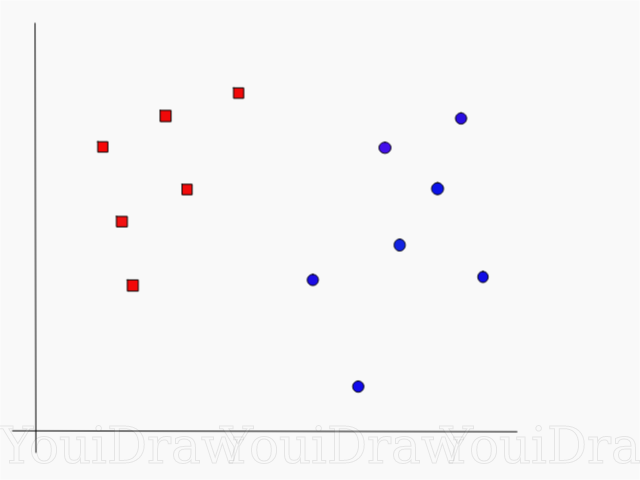
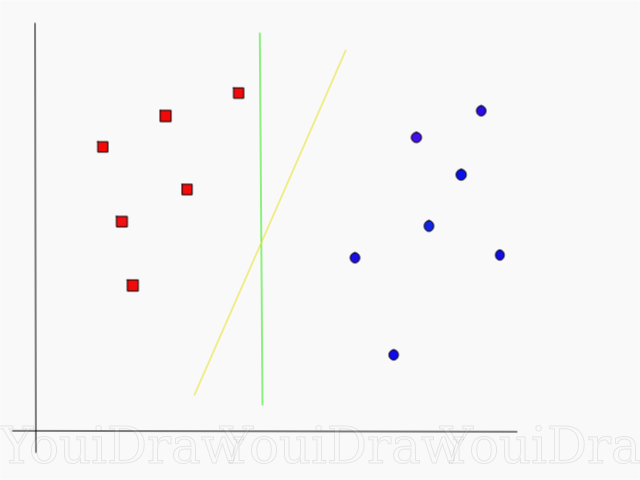
比较下面两张图：我们发现图二的决策边界更具有一般性，但是我们的模型得到的是图一中的结果，图一中蓝色的决策边界有点过拟合，因为它过于在意完全分类正确，对于左上角的一个异常样本，为了将它分类正确，导致最终的分割线严重偏斜。所以，我们希望允许SVM有错误分类，这样才能提高模型的泛化能力。

Screen Shot 2018-09-13 at 6.07.12 PM

Screen Shot 2018-09-13 at 6.07.01 PM

在上述SVM的定义中，因为我们要求所有样本点的函数间隔都要大于等于1，即每个样本点都分类正确；那么允许分类错误意味着某些样本点不满足函数间隔大于等于1的约束条件, 故可以针对每个样本点引进一个松弛变量$\xi_{i}\ge0$, 使函数间隔加上松弛变量大于等于1. 这样, 约束条件变为:

$y_i(w\dot{x_i}+b)+\xi_{i}\ge1$

同时, 对每个松弛变量$\xi_{i}$, 支付一个代价$\xi_{i}$, 则目标函数由原来的$\frac{1}{2}||w||^2$变成

$\frac{1}{2}||w||^2+C\sum_{i=1}^{N}\xi_i$

$C\ge0$称为惩罚参数. 最小化目标函数包含两层含义: 使$\frac{1}{2}||w||^2$尽量小即间隔尽量打, 同时使误分类点的个数尽量小, C是调和二者的系数. C越大，则允许的分类错误越少；C越小，则允许多的分类误差。

令$z_i=y_i(w\dot{x_i}+b)-1$时，

$l_{0/1}(z)= \left\{ \begin{align} 1, & \text{if z<0}\\ 0, &\text{otherwise} \end{align} \right.$

代入得：

$\frac{1}{2}||w||^2+C\sum_{i=1}^{N}l_{0/1}(y_i(w\dot{x_i}+b)-1)$

但是$l_{0/1}$是阶跃函数，非凸，非连续，所以我们采用其他函数来代替，替代损失函数一般选取凸的连续函数且是$l_{0/1}$的上界，常用的：

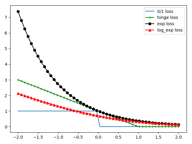
$hinge损失：l_{hinge}(z)=max(0,1-z)\\ 指数损失：l_{exp}(z)=e^{-z}\\ 对率损失：l_{log}=log(1+e^{-z})$

以上函数的x正半轴几乎为0，与我们的事实符合：$z_i=y_i(w\dot{x_i}+b)-1>0$，则没有任何损失。

则线性支持向量机的学习问题变成了如下凸二次规划问题:

$\min\limits_{w, b,\xi}\frac{1}{2}||w||^2+C\sum_{i=1}^{N}\xi_i\\ \begin{align*}s.t. &y_i(w\dot{x_i}+b)\ge1-\xi_{i}, i=1,2,...,N\\&\xi_i\ge0, i=1,2,...,m\end{align*}$

损失函数

Say given an example $(x_i,y_i)$, and use the shorthand for the scores vector: $s=f(x_i,W)$, then the SVM loss has the following form:

$L_i = \sum_{j\ne y_i}\left\{ \begin{align} 0& & \text{if } s_{y_i}\ge s_j+1 \\ s_j-s_{y_i}+1& &\text{if otherwise} \end{align} =\sum_{j\ne y_i}max(0,s_j-s_{y_i}+1) \right.$

其中，$y_i$是groundtruth label，$s_{y_i}$是分类器给真实分类的分数，$s_j$是分类器给其他类的分数，该损失函数鼓励真实分类的分数大于其他分类的分数+1。

creen Shot 2019-06-03 at 4.04.02 P

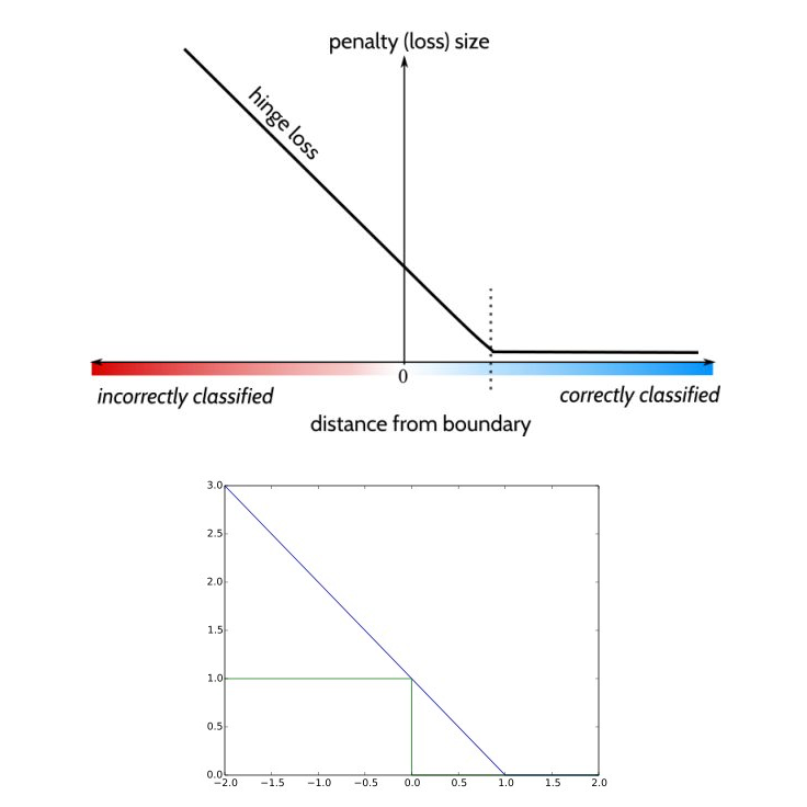
The two given figures are plots of function $f(x)=max(0,1-x)$ .We can see from the second figure that when x is between 0 and 1, the loss is in range $[0,1]$.

Examples

Say we have an image classification and we use it to classify three images, like the following:

creen Shot 2019-06-03 at 4.27.50 P

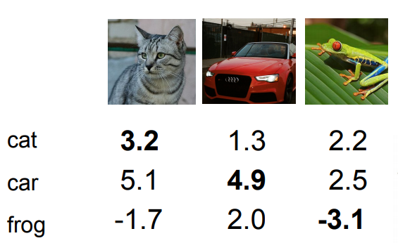
The output of classification is a 3d vector, each element of the vector is the probability of image classification. For example, for the cat image, the vector is $[3.2, 5.1, -1.7]$, meaning this picture is cat with probability 3.2, is car with prob 5.1 and frog with prob -1.7.

Then, the $s_{y_i}=3.2$, $s_1=5.1$ and $s_2=-1.7$，so the loss is:

$L_{cat}=max(0,5.1+1-3.2)+max(0,-1.7+1-3.2)=max(0,2.9)+max(0,-3.9)=2.9$

Similarily, $L_{car}=0$, $L_{frog}=12.9$.

So the overall loss is:

$L=\frac{1}{N}\sum_{i=1}^{N}L_i\\ L=\frac{(2.9+0+12.9)}{3}=5.27$

What happens to loss if car scores change a bit?

The answer is the loss will not change. The SVM loss only cares about getting the correct score to be greater than one more than the incorrect scores. But in this case, the car score is already quite a bit large than the others. So if the scores for this class changes, this margin of one will still be retained and the loss will not change.

What is the min/max possible loss?

The min loss is 0 because across all the classes, if our correct score was much larger then we will incur zero loss across all the classes.

The max loss is infinite. According to the hinge loss figure, if correct score goes very very negative, then we could incur potentially infinite loss.

At initialization W is small so all $s\approx 0$. What is the loss?

The answer is the number of class minus one.

What if the sum was over all classes?(including $j=y_j$).

The loss increases by one.

What if we used mean instead of sum?

The answer is that it doesn’t change. We just rescale the whole loss function by a constant value and we don’t care about the true value of the loss.

What if we used $L_i=\sum_{j\ne y_i}max(0,s_j-s_{y_i}+1)^2$?

The answer is it is different. We are kind of changing the trade-offs between good and badness in kind of nonlinear way, and this would end up actually computing a different loss function.

Suppose we found a W such that $L=0$. Is this W unique?

The answer is no. $2W$ is also has $L=0$.

Derivative ref

Say for a single datapoint $(x_i,y_i)$, we have the following hinge loss:

$L_i=\sum_{j\ne y_i}^{c} max(0, s_j+1-s_i)$

where $c$ is the class number and $s_j=w_j^T x_i$ is the score for the $j{th}$ class. What we do here is to iterate scores for all classes and compare them with the score of truth class.

To spread out,

$\begin{align*} L_i = &\max(0,1+w_1x_i-w_{y_i}x_i) + \\ &\max(0, 1+w_2x_i-w_{y_i}x_i) + \\ & \quad \quad \quad \quad \quad \quad \vdots \\ &\max(0, 1+w_cx_i-w_{y_i}x_i) \end{align*}$

If $(w_jx_i+1-w_{y_i}x_i)>0$, $\frac{dL_i}{dw_j}=x_i$.

But for $w_{y_i}$,

$\begin{align*} \frac{dL_i}{dw_{y_i}} &= - \sum_{j\neq y_i} \mathbb{1}(x_iw_j - x_iw_{y_i} + \Delta > 0) x_i \tag{3} \end{align*}$

Numpy Implementation

点击显/隐内容

import numpy as np

class SVM():
    def __init__(self):
        self.W = None
    def svm_loss_naive(self,W, X, y, reg):
        '''
        :param W:A numpy array of shape (D, C) containing weights.
        :param X:A numpy array of shape (N, D) containing a minibatch of data.
        :param y:A numpy array of shape (N,) containing training labels; y[i] = c means
        that X[i] has label c, where 0 <= c < C.
        :param reg:(float) regularization strength
        :return:a tuple of:
                 - loss as single float
                 - gradient with respect to weights W; an array of same shape as W
        '''
        dW = np.zeros(W.shape)
        num_classes = W.shape[1]
        num_train = X.shape[0]
        loss = 0.0
        scores = np.dot(X, W)
        for i in range(num_train):
            target = y[i]
            score = scores[i]
            for j in range(num_classes):
                if target == j:
                    continue
                if score[j] - score[target] + 1 > 0:
                    loss += score[j] - score[target] + 1
                    dW[:, j] += X[i]
                    dW[:, target] -= X[i]
        loss /= num_train
        loss += reg * np.sum(W ** 2)
        dW = dW / num_train + 2 * reg * W
        return loss, dW

    def svm_loss_vectorized(self,W, X, y, reg):
        N = np.shape(X)[0]
        C = np.shape(W)[1]
        loss = 0.0
        dW = np.zeros(W.shape)

        scores = np.dot(X, W)
        target_scores = scores[np.arange(N), y].reshape(-1, 1)
        scores_pos = scores - target_scores + 1
        scores_pos[np.arange(N), y] = 0
        scores_pos = np.maximum(scores_pos, 0)
        loss = np.sum(scores_pos) / N

        mask = np.zeros(scores_pos.shape)
        mask[scores_pos > 0] = 1
        mask[np.arange(N), y] -= np.sum(mask, axis=1)  # attention:"-"
        dW = np.dot(X.T, mask)
        dW = dW / N + 2 * reg * W

        return loss, dW

    def loss(self, X_batch, y_batch, reg):
        return self.svm_loss_vectorized(self.W, X_batch, y_batch, reg)

    def train(self, X, y, learning_rate=1e-3, reg=1e-5, num_iters=100,
              batch_size=200, verbose=False):
        '''

        :param X:A numpy array of shape (N, D) containing training data; there are N
          training samples each of dimension D.
        :param y:A numpy array of shape (N,) containing training labels; y[i] = c
          means that X[i] has label 0 <= c < C for C classes.
        :param learning_rate:(float) learning rate for optimization.
        :param reg:(float) regularization strength.
        :param num_iters:(integer) number of steps to take when optimizing
        :param batch_size:(integer) number of training examples to use at each step.
        :param verbose:(boolean) If true, print progress during optimization.
        :return:A list containing the value of the loss function at each training iteration.
        '''
        num_train, dim = X.shape
        num_classes = np.max(y) + 1  # assume y takes values 0...K-1 where K is number of classes
        if self.W is None:
            # lazily initialize W
            self.W = 0.001 * np.random.randn(dim, num_classes)

        # Run stochastic gradient descent to optimize W
        loss_history = []
        for it in range(num_iters):
            mask = np.random.choice(num_train, batch_size)
            X_batch = X[mask]
            y_batch = y[mask]

            # evaluate loss and gradient
            loss, grad = self.loss(X_batch, y_batch, reg)
            loss_history.append(loss)
            self.W -= learning_rate * grad
            if verbose and it % 100 == 0:
                print('iteration %d / %d: loss %f' % (it, num_iters, loss))
        return loss_history

    def predict(self, X):
        y_pred = np.zeros(X.shape[0])
        scores = X.dot(self.W)
        y_pred = np.argmax(scores,axis=1)
        return y_pred

核方法

引言

通俗说，只要涉及空间的变换和內积的运算，我们就可以使用Kernel trick来简化运算。

一般的，在高维空间计算內积，我们需要分两步：

将原始低维数据空间$X$映射到更高维的$Z$空间：
$\phi(x):X\to Z$
在$Z$空间里计算內积：
$z_i = \phi(x_i)\\ z_j = \phi(x_j)\\ k = z_i^Tz_j$

而核方法：

$K(x_i,x_j)=z_i^Tz_j=\phi(x_i)^T\phi(x_j)$

即，$K(x_i,x_j)$计算得到的结果就是原始数据空间中的两点先升维$\phi(x)$再內积$\phi(x_i)^T\phi(x_j)$的结果，不必进行显示的升维操作。

Kernel Trick in SVM

kernel visualiztion

那么SVM中如何利用核方法呢？且看下面的这个例子。

Screen Shot 2018-09-15 at 10.42.27 PM (2) .png)

在一维空间（直线上）我们有一系列样本点，蓝色为正例，红色为负例，显然我们不能找到一个线性的分割来分类它们。那么，如果将一维的数据点映射到二维平面呢？即对每个样本点，我们先进行映射：$(x)\to (x,y)$，其中$y=x^2$，这样就将蓝色和红色的样本点分开了，于是，我们就可以使用一条直线取划分样本点了。

再看一个二维空间的例子，如下图所示：

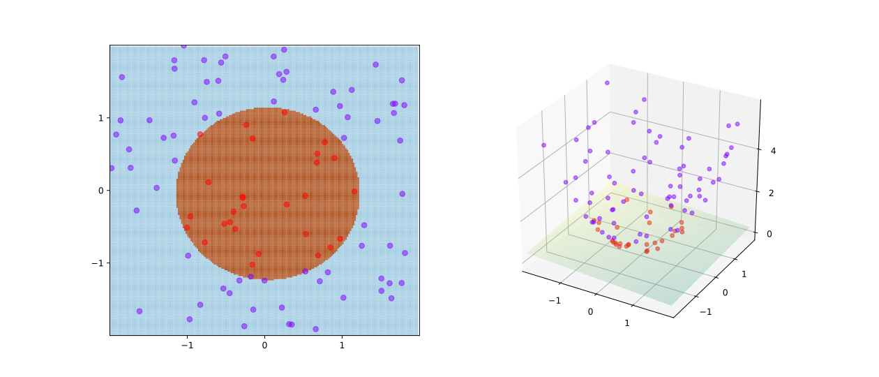
显然我们无法使用线性的分割去分类上述点，但是如果我们将二维平面上的点增加一个维度$z$，使平面上点映射到三维空间上，$(x,y)\to (x,y,z)$，如右边图所示，这样我们就可以使用一个平面进行划分了。

常用核函数

通过上面的讨论，我们希望样本在新的特征空间内线性可分，因此特征空间的好坏对支持向量机的性能至关重要。但是在不知道特征映射的形式时，我们并不知道什么样的核函数是合适的，而核函数也仅是隐式地定义了这个特征空间，故选择合适的核函数很重要。

线性核：$k(x_i,x_j)=x_i^Tx_j$
多项式核：$k(x_i,x_j)=(\gamma x_i^Tx_j+r)^d$

当$d>1$
高斯核：$k(x_i,x_j)=e^{(-\frac{||x_i-x_j||^2}{2\sigma^2})}$

亦称RBF核，$\sigma>0$为高斯核的带宽

如果$\sigma$设的太小，方差会很小，方差很小的高斯分布长得又高又瘦，会造成只会作用于支持向量样本附近，对于未知样本分类效果很差，存在训练准确率可以很高，(如果让方差无穷小，则理论上，高斯核的SVM可以拟合任何非线性数据，但容易过拟合)而测试准确率不高的可能，就是通常说的过训练；而如果设的过大，则会造成平滑效应太大，无法在训练集上得到特别高的准确率，也会影响测试集的准确率。ref
拉普拉斯核：$k(x_i,x_j)=e^{(-\frac{||x_i-x_j||^2}{\sigma^2})}$

$\sigma>0$
Sigmoid核：$k(x_i,x_j)=tanh(\beta x_i^Tx_j+\theta)$

$\beta>0$，$\theta<0$

Python

import numpy as np
X = np.array([[-1, -1], [-2, -1], [1, 1], [2, 1]])
y = np.array([1, 1, 2, 2])
from sklearn.svm import SVC
clf = SVC(kernel='linear')
clf = SVC.fit(X, y)
prediction = clf.predict([[0,6]])

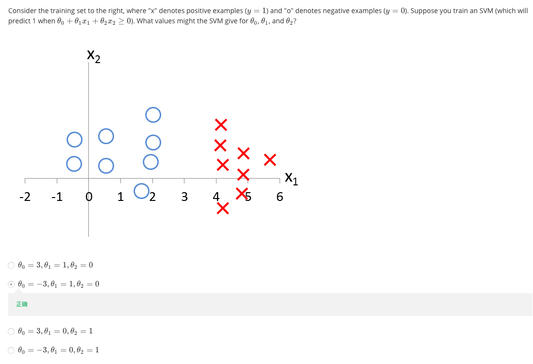
Exercise1

Machine Learning Exercises In Python, Part 6 - SVM

Screen Shot 2018-09-11 at 10.16.55 AM

Screen Shot 2018-09-11 at 9.44.08 AM