Several metrics to evaluate GAN, including Inception Score.

Motivation

Consider this setting: a zoo of GANs you’ve trained has generated several sets of images: $X_1, X_2, …, X_N$ that are trying to mimic the original set $X_{real}$. If you had a perfect way to rank the realism if these sets, let’s say, a function $\rho(X)$, then $\rho(X_{real})$ would, obviously, be the highest of all. The real question is:

How can such function be formulated in terms of statistics / information theory?

The answer depends on the requirements for the images. Two criteria immediately come to mind:

A human, looking at a separate image, would be able to confidently determine what’s in there (saliency).
A human, looking at a set of various images, would say that the set has lots of different objects (diversity).

At least, that’s what everyone expects from a good generative model. Those who have tried training GANs themselves have immediately noted the fact that usually you end up getting only one criterion covered.

Saliency vs. diversity

Broadly speaking, these two criteria are represented by two components of the formula:

Saliency is expressed as $p(y|x)$ — a distribution of classes for any individual image should have low entropy (think of it as a single high score and the rest very low).
Diversity is expressed is $p(x)$ — overall distribution of classes across the sampled data should have high entropy, which would mean the absense of dominating classes and something closer to a well-balanced training set.

Kullback-Leibler distance ref

Since we are going to explain the KL divergence from the information theory point of view, let us review what is entropy and cross-entropy.

Entropy and Cross-Entropy ref

First of all, we need to know Surprisal: Degree to which you are surprised to see the result. This means we will be more surprised to see an outcome with low probability in comparison to an outcome with high probability. Now, if $y_i$ is the probability of ith outcome then we could represent surprisal (s) as:

$s=-\log \left( y_{i}\right)$

Entropy

Since I know surprisal for individual outcomes, I would like to know surprisal for the event. It would be intuitive to take a weighted average of surprisals. Now the question is what weight to choose? Hmmm…since I know the probability of each outcome, taking probability as weight makes sense because this is how likely each outcome is supposed to occur. This weighted average of surprisal is nothing but Entropy (e) and if there are noutcomes then it could be written as:

$e=\sum_{0}^{n} y_{i} \log \left(1 / y_{i}\right)$

Cross-Entropy

Now, what if each outcome’s actual probability is $p_i$ but someone is estimating probability as $q_i$. In this case, each event will occur with the probability of $p_i$ but surprisal will be given by $q_i$ in its formula (since that person will be surprised thinking that probability of the outcome is $q_i$). Now, weighted average surprisal, in this case, is nothing but cross entropy(c) and it could be scribbled as:

$c=\sum_{0}^{n} p_{i} \log \left(1 / q_{i}\right)$

Cross-entropy is always larger than entropy and it will be same as entropy only when $p_i=q_i$. You could digest the last sentence after seeing really nice plot given by desmos.com

Cross-Entropy Loss

_NJTe1lQSz21vQU0xX0PLm

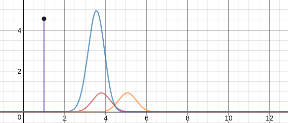
In the plot I mentioned above, you will notice that as estimated probability distribution moves away from actual/desired probability distribution, cross entropy increases and vice-versa. Hence, we could say that minimizing cross entropy will move us closer to actual/desired distribution and that is what we want. This is why we try to reduce cross entropy so that our predicted probability distribution end up being close to the actual one. Hence, we get the formula of cross-entropy loss as:

$c=\sum_{0}^{n} p_{i} \log \left(1 / q_{i}\right)$

And in the case of binary classification problem where we have only two classes, we name it as binary cross-entropy loss and above formula becomes:

$c=\sum_{0}^{1} p_{i} \log \left(1 / q_{i}\right)=p_{0} \log \left(1 / q_{0}\right)+p_{1} \log \left(1 / q_{1}\right)=p_{0} \log \left(1 / q_{0}\right)+\left(1-p_{0}\right) \log \left(1 /\left(1-q_{0}\right)\right)$

Kullback-Leibler distance

The KL divergence tells us how well the probability distribution $Q$ approximates the
probability distribution $P$ by calculating the cross-entropy minus the entropy.

$D_{K L}(P \| Q)=H(P, Q)-H(P)$

As a reminder, I put the cross-entropy and the entropy formula as below:

$\begin{aligned} H(P, Q) &=\mathbb{E}_{x \sim P}[-\log Q(x)] \\ H(P) &=\mathbb{E}_{x \sim P}[-\log P(x)] \end{aligned}$

The KL divergence can also be expressed in the expectation form as follows:

$\begin{aligned} D_{K L}(P \| Q) &=\mathbb{E}_{x \sim P}[-\log Q(x)]-\mathbb{E}_{x \sim P}[-\log P(x)] \\ &=\mathbb{E}_{x \sim P}[-\log Q(x)-(-\log P(x))] \\ &=\mathbb{E}_{x \sim P}[-\log Q(x)+\log P(x)] \\ &=\mathbb{E}_{x \sim P}[\log P(x)-\log Q(x)] \\ &=\mathbb{E}_{x \sim P}\left[\log \frac{P(x)}{Q(x)}\right] \end{aligned}$

The expectation formula can be expressed in the discrete summation form or in the
continuous integration form:

$\begin{aligned} D_{K L}(P \| Q) &=\sum_{i} P(i) \log \frac{P(i)}{Q(i)} \\ D_{K L}(P \| Q) &=\int P(x) \log \frac{P(x)}{Q(x)} d x \end{aligned}$

So, what does the KL divergence measure? It measures the similarity (or dissimilarity)
between two probability distributions.

KL divergence is non-negative

The KL divergence is non-negative. An intuitive proof is that:

if $P=Q$, the KL divergence is zero as:

$log \frac{P}{Q} = log1=0$

if $P \ne Q$, the KL divergence is positive because the entropy is the minimum average
lossless encoding size.

So, the KL divergence is a non-negative value that indicates how close two probability
distributions are.

KL devergence is asymmetric

The KL divergence is not symmetric: $D_{KL}(P||Q)\ne D_{KL}(Q||P)$.

It can be deduced from the fact that the cross-entropy itself is asymmetric. The crossentropy $H(P, Q)$ uses the probability distribution $P$ to calculate the expectation. The
cross-entropy $H(Q, P)$ uses the probability distribution $Q$ to calculate the expectation.
So, the KL divergence cannot be a distance measure as a distance measure should be
symmetric.

Modeling a true distribution

By approximating a probability distribution with a well-known distribution like the
normal distribution, binomial distribution, etc., we are modeling the true distribution
with a known one.
This is when we are using the below formula:

$D_{K L}(P \| Q)=\mathbb{E}_{x \sim P}\left[\log \frac{P(x)}{Q(x)}\right]$

Calculating the KL divergence, we can find the model (the distribution and the
parameters) that fits the true distribution well.

And that’s it. One important thing to keep in mind (and, actually, the most fascinating among these), is that to compute this score for a set of generated images you need a good image classifier. Hence the name of the metric — for calculating the distributions the authors used a pretrained Inception.

Higher Inception score indicates better image quality.

Implementation

import math
import torch
import torch.nn.functional as F
from torch.autograd import Variable
from torchvision.models import inception_v3

net = inception_v3(pretrained=True).cuda()
def inception_score(images, batch_size=5):
    scores = []
    for i in range(int(math.ceil(float(len(images)) / float(batch_size)))):
        batch = Variable(torch.cat(images[i * batch_size: (i + 1) * batch_size], 0))
        s, _ = net(batch)  # skipping aux logits
        scores.append(s)
    p_yx = F.softmax(torch.cat(scores, 0), 1)
    p_y = p_yx.mean(0).unsqueeze(0).expand(p_yx.size(0), -1)
    KL_d = p_yx * (torch.log(p_yx) - torch.log(p_y))
    final_score = KL_d.mean()
    return final_score

keras-implementation

Inception Score 的原理和局限性

Fréchet Inception Distance

ref1 Fréchet Inception Distance (FID)

The FID is supposed to improve on the IS by actually comparing the statistics of generated samples to real samples, instead of evaluating generated samples in a vacuum.

$\text{FID} = ||\mu_r - \mu_g||^2 + \text{Tr} (\Sigma_r + \Sigma_g - 2 (\Sigma_r \Sigma_g)^{1/2}),$

where $X_r \sim \mathcal{N} (\mu_r, \Sigma_r)$ and $X_g \sim \mathcal{N} (\mu_g, \Sigma_g)$ are the 2048-dimensional activations of the Inception-v3 pool3 layer for real and generated samples respectively. Lower FID is better, corresponding to more similar real and generated samples as measured by the distance between their activation distributions.

implementation

SSD-Score

Implementation

ref1