Recurrent Neural Networks, which are a type of artificial neural network designed to recognize patterns in sequences of data, such as text, genomes, handwriting, the spoken word, or numerical times series data emanating from sensors, stock markets and government agencies. These algorithms take time and sequence into account, they have a temporal dimension.
Problems with Vanilla NN link
A glaring limitation of Vanilla Neural Networks (and also Convolutional Networks) is that their API is too constrained: they accept a fixed-sized vector as input (e.g. an image) and produce a fixed-sized vector as output (e.g. probabilities of different classes).
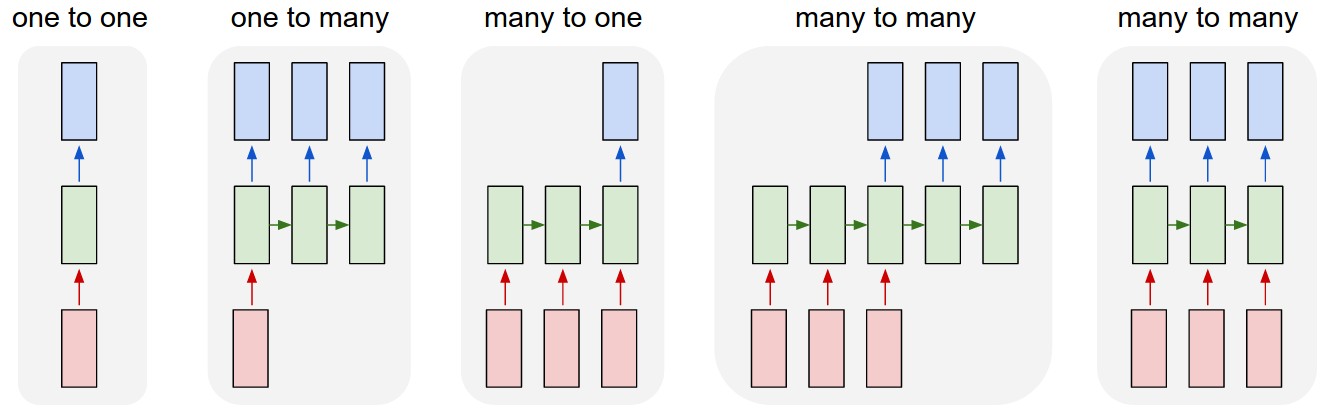
Each rectangle is a vector and arrows represent functions (e.g. matrix multiply). Input vectors are in red, output vectors are in blue and green vectors hold the RNN’s state (more on this soon). From left to right: (1) Vanilla mode of processing without RNN, from fixed-sized input to fixed-sized output (e.g. image classification). (2) Sequence output (e.g. image captioning takes an image and outputs a sentence of words). (3) Sequence input (e.g. sentiment analysis where a given sentence is classified as expressing positive or negative sentiment). (4) Sequence input and sequence output (e.g. Machine Translation: an RNN reads a sentence in English and then outputs a sentence in French). (5) Synced sequence input and output (e.g. video classification where we wish to label each frame of the video). Notice that in every case are no pre-specified constraints on the lengths sequences because the recurrent transformation (green) is fixed and can be applied as many times as we like.
RNN
At a high level, a recurrent neural network (RNN) processes sequences — whether daily stock prices, sentences, or sensor measurements — one element at a time while retaining a memory (called a state) of what has come previously in the sequence.
A Gentle Tutorial of Recurrent Neural Network with Error Backpropagation
given an observation sequence $\mathbf{x}=\left\{\mathbf{x}_{1}, \mathbf{x}_{2}, \ldots, \mathbf{x}_{T}\right\}$ and its corresponding label $y=\left\{y_{1}, y_{2}, \ldots, y_{T}\right\}$, we want to learn a map $f : \mathbf{x} \mapsto y$.
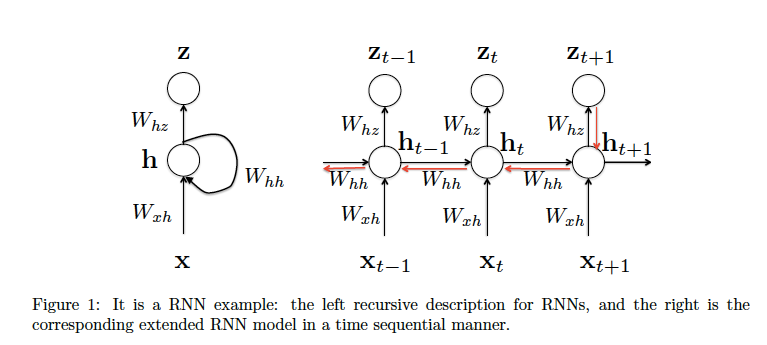
Suppose that we have the following RNN model, such that
where $z_t$ is the prediction at the time step $t$.
We can minimize the negative log likelihood objective function:
In the following, we will use notation $L$ as the objective function for simplicity. And further we will use $L(t + 1)$ to indicate the output at the time step t + 1, s.t. $L(t + 1) = -y_{t+1}logz_{t+1}$.
Let’s set $\alpha_{t}=W_{h z} \mathbf{h}_{t}+\mathbf{b}_{z}$ and then we have $z_t=softmax(\alpha_t)$. By taking the derivative with respect to $ \alpha_t$, we get the following:
Note the weight $W_{hz}$ is shared across all time sequence, thus we can dierentiate to it at each time
step and sum all together
Similarly, we can get the gradient w.r.t. bias $b_z$
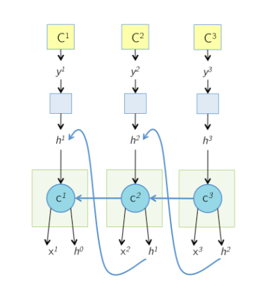
Now let’s go through the details to derive the gradient w.r.t. $W_{hh}$. Considering at the time step $t \to t+1$ in figure1,
where we only consider one step $t \to t+1$. And because the hidden state $h_{t+1}$ partially dependents
on $h_t$, so we can use backpropagation to compute the above partial derivative. Think further $W_{hh}$ is shared cross the whole time sequence. Thus, at the time step $(t -1) \to t$, we can further get the partial derivative w.r.t. $W_{hh}$ as follows
Thus, at the time step $t+1$, we can compute gradient w.r.t. $z_{t+1}$ and further use backpropagation
through time (BPTT) from t to 0 to calculate gradient w.r.t. $W_{hh}$, shown as the red chain in Fig. 1.
Thus, if we only consider the output $z_{t+1}$ at the time step $t+1$, we can yield the following gradient
w.r.t. $W_{hh}$
Aggregate the gradients w.r.t. $W_{hh}$ over the whole time sequence with back propagation, we can
finally yield the following gradient w.r.t. $W_{hh}$
Now we turn to derive the gradient w.r.t. $W_{xh}$. Similarly, we consider the time step $t + 1$ (only
contribution from $x_{t+1}$) and calculate the gradient w.r.t. to $W_{xh}$ as follows
Because $h_t$ and $x_{t+1}$ both make contribution to $h_{t+1}$, we need to backpropagte to $h_t$ as well. If we
consider the contribution from the time step $t$, we can further get
Thus, summing up all contributions from $t$ to 0 via backpropagation, we can yield the gradient at
the time step $t + 1$
Further, we can take derivative w.r.t. $W_{xh}$ over the whole sequence as
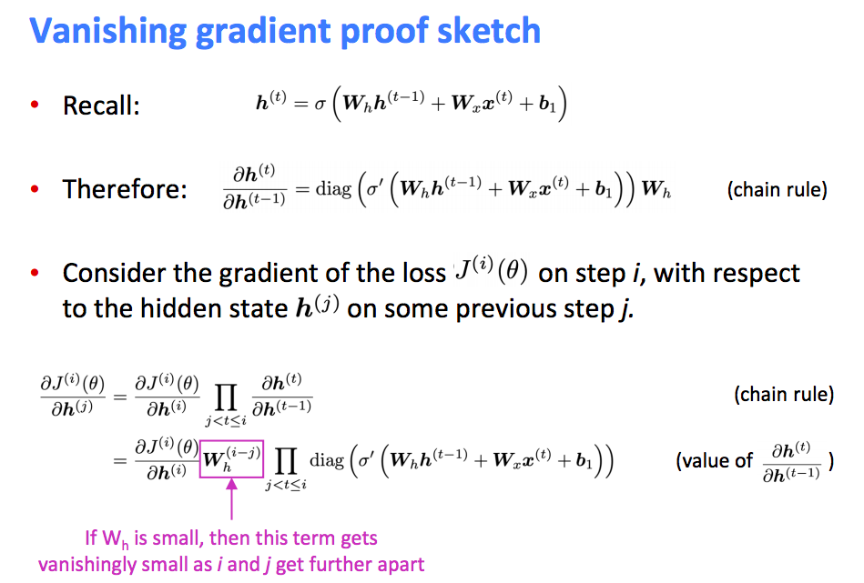
However, there are gradient vanishing or exploding problems to RNNs. Notice that $\frac{\partial \mathbf{h}_{t+1}}{\partial \mathbf{h}_{k}}$ indicates matrix multiplication over the sequence. Because RNNs need to backpropagate gradients over a long sequence (with small values in the matrix multiplication), gradient value will shrink layer over layer, and eventually vanish after a few time steps. Thus, the states that are far away from the current time step does not contribute to the parameters’ gradient computing (or parameters that RNNs is learning). Another direction is the gradient exploding, which attributed to large values in matrix multiplication.
Forward propagation
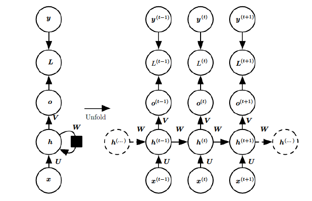
$x$: input, $h$: hidden layer, $o$: output, $y$: target label, $L$: loss function, $t$: time
At time t, we have hidden state:
where $\phi()$ is activation function, typically $tanh()$, and $b$ is the bias.
The output is at time t is:
Then the prediction is:
where $\sigma()$ is the activation function, typically $softmax()$.
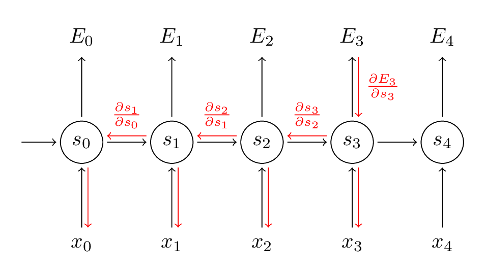
Back Propagation through Time
Let’s quickly recap the basic equations of our RNN.
We also defined our loss, or error, to be the cross entropy loss, given by:
Here, $y_t$ is the correct word at time step $t$, and $\hat y_t$ is our prediction. We typically treat the full sequence (sentence) as one training example, so the total error is just the sum of the errors at each time step (word).
Remember that our goal is to calculate the gradients of the error with respect to our parameters $U$, $V$ and $W$.
In the above, $z_{3}=V s_{3}$ and $\oplus$ is the outer product of two vectors. We can find that $\frac{\partial E_{3}}{\partial V}$ only depends on the values at the current time step, $\hat{y}_{3}, y_{3}, s_{3}$.
But the story is different for $\frac{\partial E_{3}}{\partial W}$ (and for $U$). To see why, we write out the chain rule, just as above:
Now, note that $s_{3}=\tanh \left(U x_{t}+W s_{2}\right)$ depends on $s_2$, which depends on $W$ and $s_1$, and so on. So if we take the derivative with respect to $W$ we can’t simply treat $s_2$ as a constant! We need to apply the chain rule again and what we really have is this:
We sum up the contributions of each time step to the gradient. In other words, because $W$ is used in every step up to the output we care about, we need to backpropagate gradients from $t=3$ through the network all the way to $t=0$.
Hand-Written RNN
hand-writtrn-deduction-1 hand-writtrn-deduction-2
Here I am going to give an simple problem about how RNN can be used to solve problems and aim to have a better understanding of how forward and backward propagation in RNN work.
Anyways here we go. The problem is very simple, we are going to use RNN to count how many ones there are in the given data.
As seen above, the training data is $x$ and $y$ is the groundtruth.
The corresponding RNN architecture looks like the following:
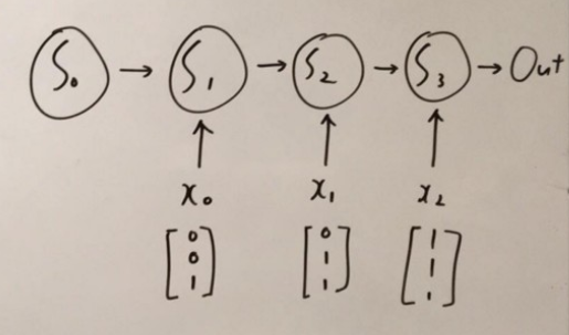
which is the unrolled version of our network architecture.
For this network, we have two weight matrixs, $W_x$ and $W_{rec}$, and the forward propagation is:
We define the MSE loss function:
Now lets perform back propagation through time. We have to get derivative respect to $W_x$ and $W_{rec}$ for each state.
State3:
State2:
State1:
So that’s it! The simple math behind training RNN.
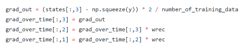
Numpy Implementation
|
|
|
|
|
|
|
|
RNN Vanishing Gradients Problem
What is gradients vanishing?
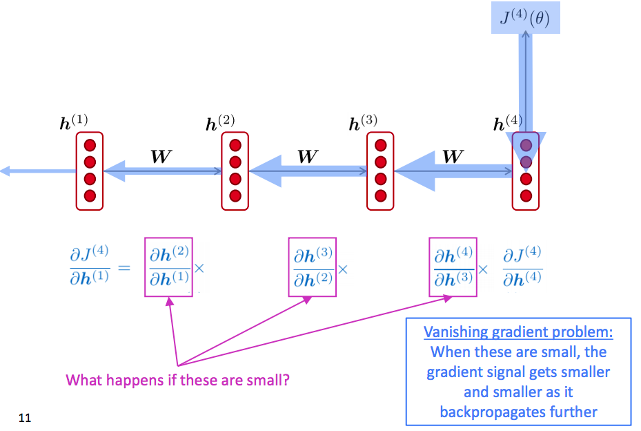
Why it is a problem?
The information from long-term timesteps is gone.
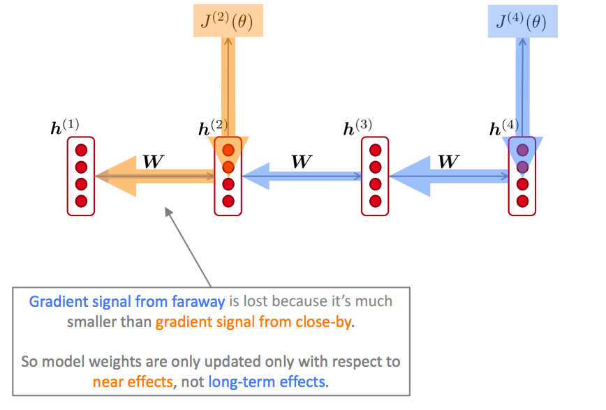
If the gradient becomes vanishingly small over longer distances (step t to step t+n), then we can’t tell whether:
- There’s no dependency between step t and t+n in the data
- We have wrong parameters to capture the true dependency between t and t+n
Long Short Term Memory networks
It is usually just called “LSTMs” – are a special kind of RNN, capable of learning long-term dependencies.
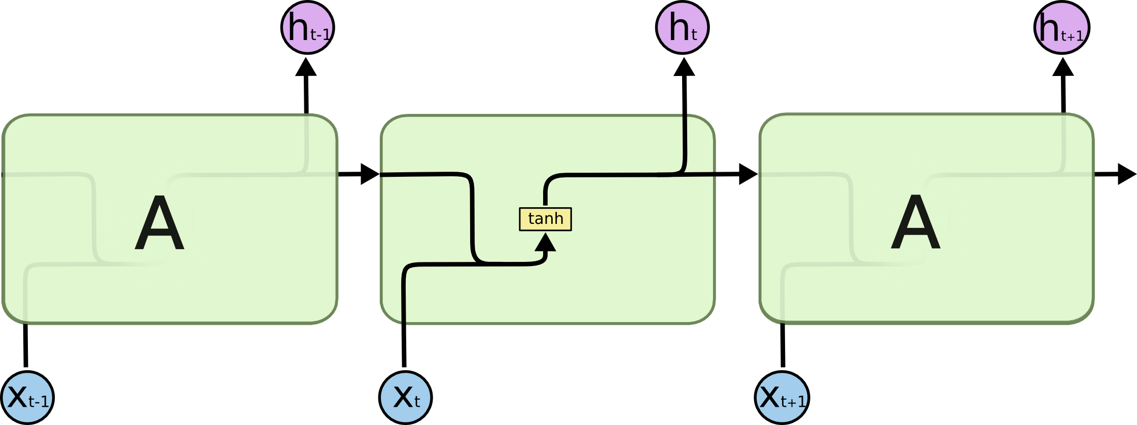
All recurrent neural networks have the form of a chain of repeating modules of neural network. In standard RNNs, this repeating module will have a very simple structure, such as a single tanh layer.
LSTMs also have this chain like structure, but the repeating module has a different structure. Instead of having a single neural network layer, there are four, interacting in a very special way.
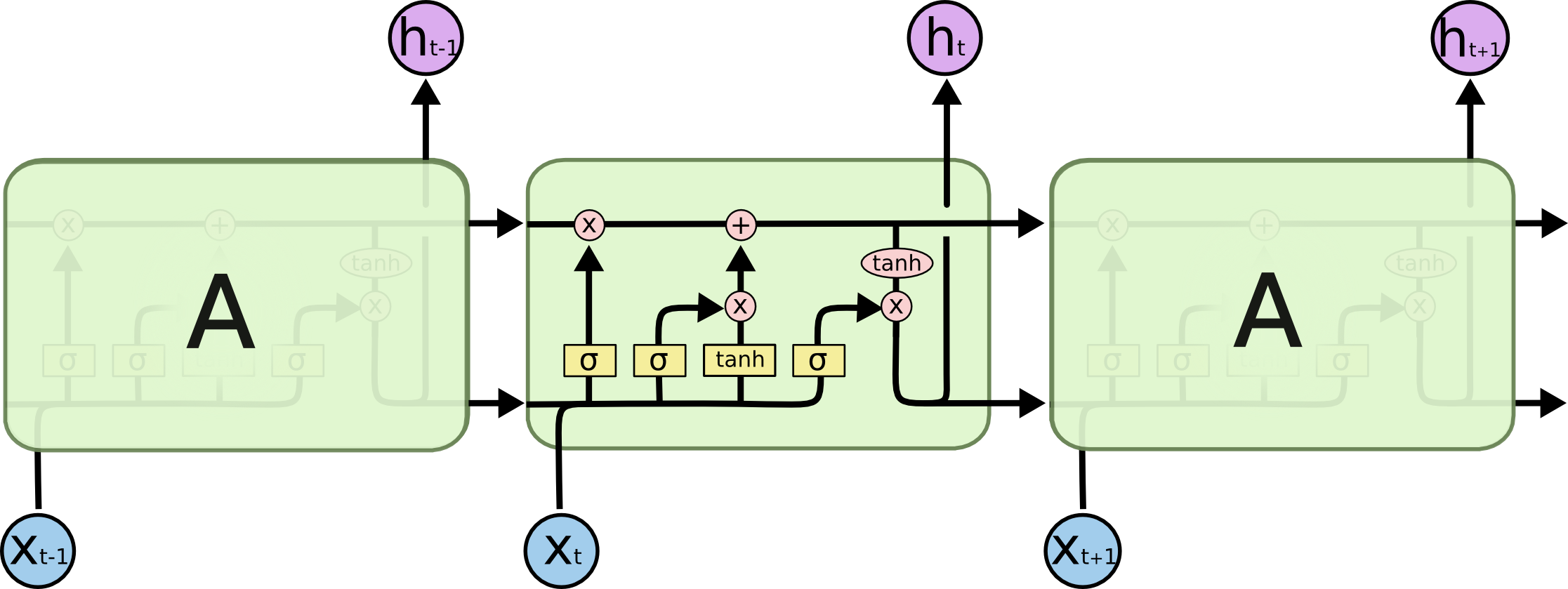
For now, let’s just try to get comfortable with the notation we’ll be using.
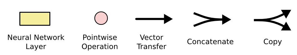
In the above diagram, each line carries an entire vector, from the output of one node to the inputs of others. The pink circles represent pointwise operations, like vector addition, while the yellow boxes are learned neural network layers. Lines merging denote concatenation, while a line forking denote its content being copied and the copies going to different locations.
The core idea behind LSTMs
The key to LSTMs is the cell state, the horizontal line running through the top of the diagram.
The cell state is kind of like a conveyor belt. It runs straight down the entire chain, with only some minor linear interactions. It’s very easy for information to just flow along it unchanged.
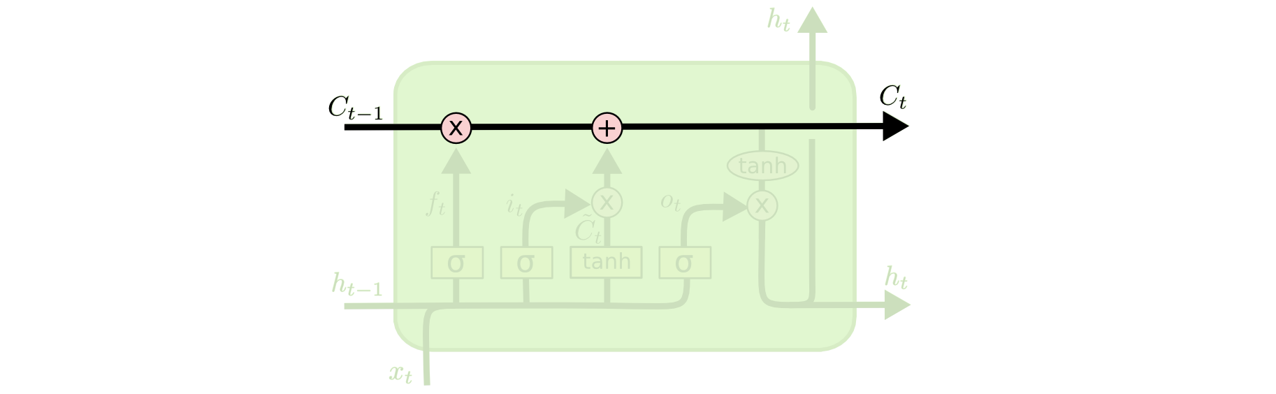
The LSTM does have the ability to remove or add information to the cell state, carefully regulated by structures called gates.
Gates are a way to optionally let information through. They are composed out of a sigmoid neural net layer and a pointwise multiplication operation.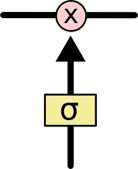
The sigmoid layer outputs numbers between zero and one, describing how much of each component should be let through. A value of zero means “let nothing through,” while a value of one means “let everything through!” An LSTM has three of these gates, to protect and control the cell state.
Step-by-Step LSTM Walk Through
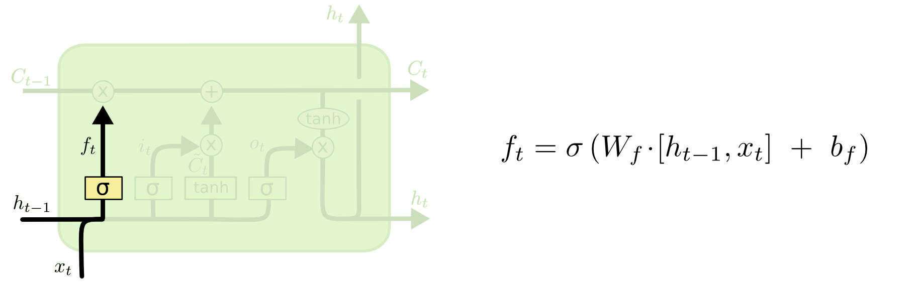
The first step in our LSTM is to decide what information we’re going to throw away from the cell state. This decision is made by a sigmoid layer called the “forget gate layer.” It looks at ht−1ht−1and xtxt, and outputs a number between 00 and 11 for each number in the cell state Ct−1Ct−1. A 11represents “completely keep this” while a 00 represents “completely get rid of this.”
Let’s go back to our example of a language model trying to predict the next word based on all the previous ones. In such a problem, the cell state might include the gender of the present subject, so that the correct pronouns can be used. When we see a new subject, we want to forget the gender of the old subject.
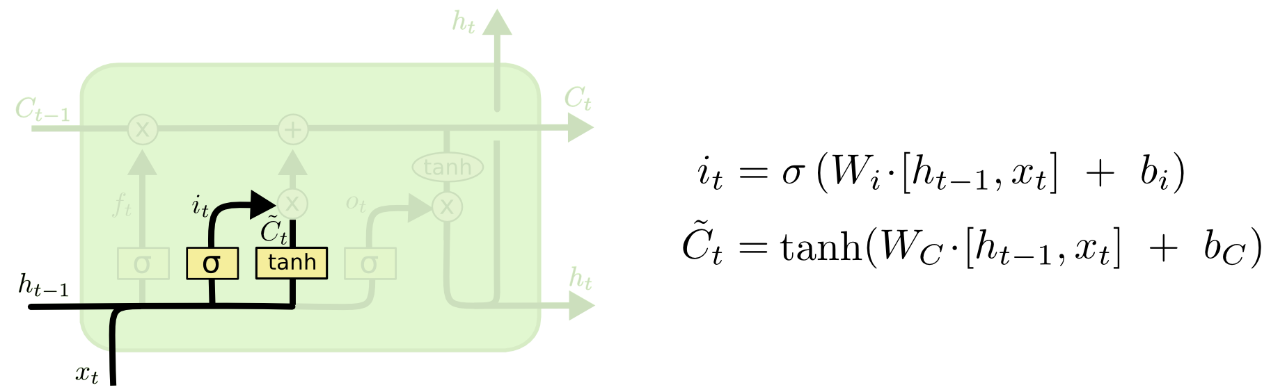
The next step is to decide what new information we’re going to store in the cell state. This has two parts. First, a sigmoid layer called the “input gate layer” decides which values we’ll update. Next, a tanh layer creates a vector of new candidate values, $\tilde C$, that could be added to the state. In the next step, we’ll combine these two to create an update to the state.
In the example of our language model, we’d want to add the gender of the new subject to the cell state, to replace the old one we’re forgetting.
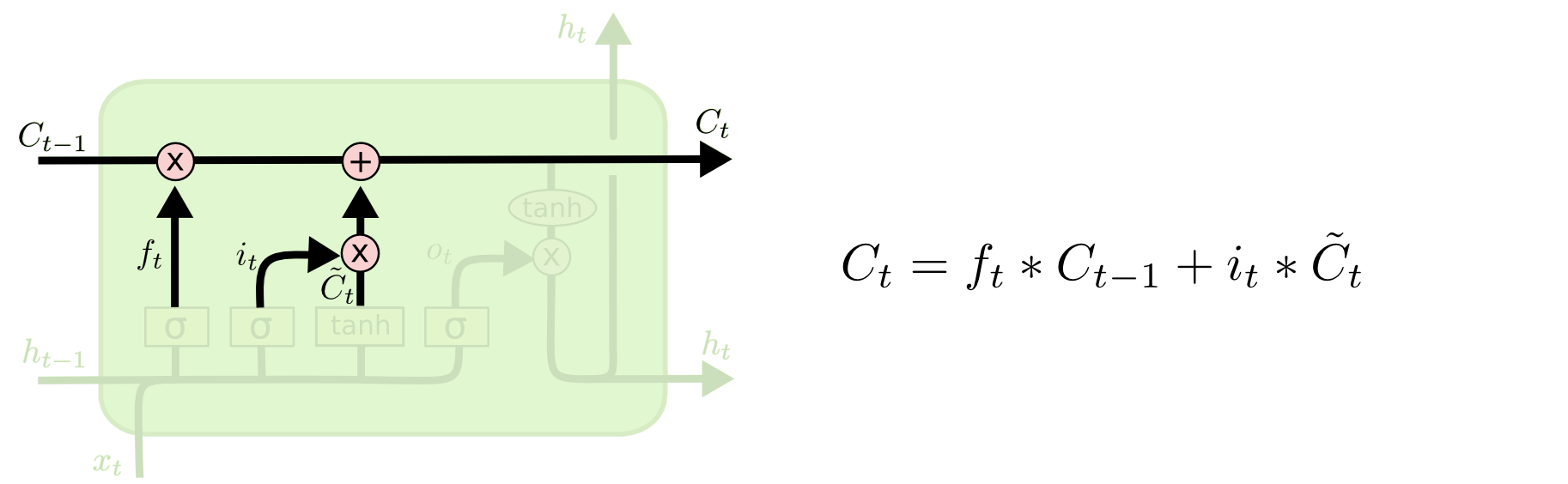
It’s now time to update the old cell state, $C_{t-1}$, into the new cell state $C_t$. The previous steps already decided what to do, we just need to actually do it.
We multiply the old state by $f_t$, forgetting the things we decided to forget earlier. Then we add $i_t* \tilde C_{t}$.
This is the new candidate values, scaled by how much we decided to update each state value.
In the case of the language model, this is where we’d actually drop the information about the old subject’s gender and add the new information, as we decided in the previous steps.
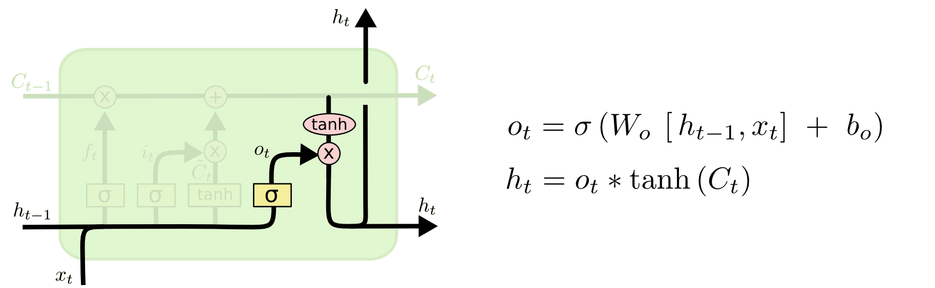
Finally, we need to decide what we’re going to output. This output will be based on our cell state, but will be a filtered version. First, we run a sigmoid layer which decides what parts of the cell state we’re going to output. Then, we put the cell state through tanh (to push the values to be between -1 and 1) and multiply it by the output of the sigmoid gate, so that we only output the parts we decided to.
For the language model example, since it just saw a subject, it might want to output information relevant to a verb, in case that’s what is coming next. For example, it might output whether the subject is singular or plural, so that we know what form a verb should be conjugated into if that’s what follows next.
Backpropagation
Recall that the forward pass of LSTM is like:

The unrolled network during the forward pass is shown above. The cell state at time T, $c^T$ is responsible for computing h as well as the next cell state $c^{T+1}$. At each time step, the cell output h is shown to be passed to some more layers on which cost function C is computed, as the way an LSTM would be used in a typical application like captioning or language modeling. source
The unrolled network during the backward pass is shown below. All the arrows in the previous slide have now changed their direction. The cell state at time T, $c^{T}$ receive gradients from $h^T$ as well as the next cell state $c^{T+1}$.
Note that for the last node, since it dosen’t have a next time stamp, it receive no gradients from $c^{T+1}$ and $h^T$, which means $d_{next_state} = 0$ and $d_{next_hidden}=0$.
Numpy Implementation
|
|
|
|
|
|
|
|
GRU
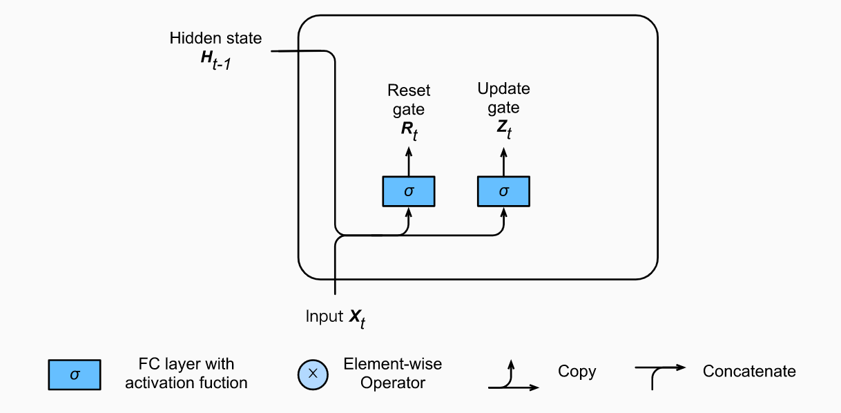
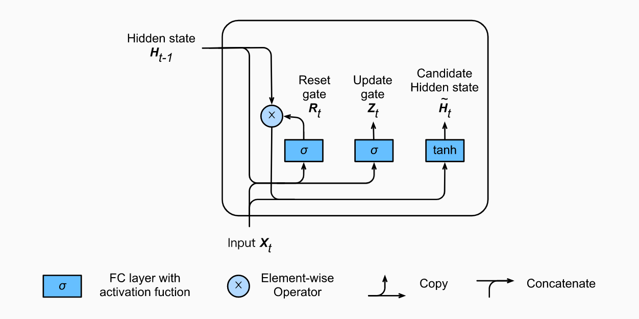
So now we know how an LSTM work, let’s briefly look at the GRU. The GRU is the newer generation of Recurrent Neural networks and is pretty similar to an LSTM. GRU’s got rid of the cell state and used the hidden state to transfer information. It also only has two gates, a reset gate and update gate.
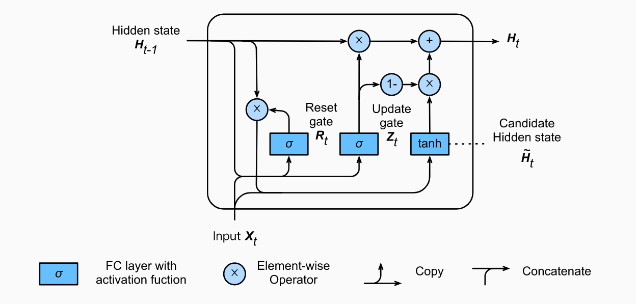
Reset Gate
How LSTM/GRU Solve Vanishing Gradients
In order to understand this question, we need to introdcue shortcut firstly. In ResNet, the shortcut is like:
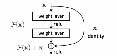
which is $x^{(t)}=x^{(t-1)}+F(x^{(t-1)})$. The next output is the combination of two parts: shortcut($x^{(t-1)}$) and non-linear transformation of $x^{(t-1)}$. Because of the shortcut, there is always a “1” gradient flowing back in backpropagation. In some extent, it sovles the problem of vanishing gradient.
Now back to our fancy RNN, take GRU as example, the updating rules of GRU is:
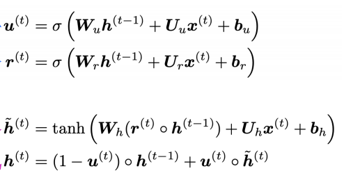
Let’s focus on how we get the new hidden state $h^{(t)}$ and let’s roll out the formulation:
which is very similar to the ResNet becasue there is a direct flow from previous state to the next state.
Keras - Learn the Alphabet
In this implementation, we are going to develop and constrast a number of different LSTM networks. The task we are going to perform is that given a letter of the alphabet, predict the next letter. This is a simple sequence prediction problem that once understood can be generalized to other sequence prediction problems like time series prediction and sequence classification.
Data Preparation
|
|
Because neural network can only process number, we map the letters to integer value.
|
|
Here, we create our input dataset and corresponding output dataset; we use an input length of 1. Running the code will produce the following output:
|
|
Then, we need to reshape our data into a format expected by the LSTM networks, that is, [data_size,time_steps,feature_num]. Then we can normalize the input integers to the range [0,1]. Finally, we can think of this problem as a sequence classification task, where each of the 26 letters represents a different class. As such, we can convert the output (y) to a one hot encoding, using the Keras built-in function to_categorical().
|
|
One-Char to One-Char
Let’s start off by designing a simple LSTM to learn how to predict the next character in the alphabet given the context of just one character.
Let’s define an LSTM network with 32 units and an output layer with a softmax activation function for making predictions. Because this is a multi-class classification problem, we can use the log loss function (called “categorical_crossentropy” in Keras), and optimize the network using the ADAM optimization function.
|
|
After we fit the model we can evaluate and summarize the performance on the entire training dataset.
|
|
We can then re-run the training data through the network and generate predictions, converting both the input and output pairs back into their original character format to get a visual idea of how well the network learned the problem.
|
|
|
|
We can see that this problem is indeed difficult for the network to learn. The reason is, the poor LSTM units do not have any context to work with. Each input-output pattern is shown to the network in a random order and the state of the network is reset after each pattern (each batch where each batch contains one pattern). This is abuse of the LSTM network architecture, treating it like a standard multilayer Perceptron. Next, let’s try a different framing of the problem in order to provide more sequence to the network from which to learn.
A Three-Char Feature Window to One-Char Mapping
A popular approach to adding more context to data for multilayer Perceptrons is to use the window method. We can do this by increasing the input sequence length length from 1 to 3, for example:seq_length=3, which creates training patterns like:
|
|
Each element in the sequence is then provided as a new input feature to the network. This requires a modification of how the input sequences reshaped in the data preparation step:
|
|
The entire code is provided below for completeness.
|
|
|
|
We can see a little improvement in the performance that may or may not be true.
Again, this is a misuse of the LSTM network by a poor framing of the problem. Indeed, the sequences of letters are time steps of one feature rather than one time step of separate features. We have given more context to the network, but not more sequence as it expected.
In the next section, we will give more context to the network in the form of time steps.
A Three-Char Time Step Window to One-Char Mapping
We still take as input a sequence with length being 3, seq_length=3. The difference is that the reshaping of the input data takes the sequence as a time step sequence of one feature, rather than a single time step of multiple features.
|
|
This is the correct intended use of providing sequence context to your LSTM in Keras. The full code example is provided below for completeness.
|
|
|
|
We can see that the model learns the problem perfectly as evidenced by the model evaluation and the example predictions.
LSTM State Within A Batch
The Keras implementation of LSTMs resets the state of the network after each batch.
This suggests that if we had a batch size large enough to hold all input patterns and if all the input patterns were ordered sequentially, that the LSTM could use the context of the sequence within the batch to better learn the sequence.
We can demonstrate this easily by modifying the first example for learning a one-to-one mapping and increasing the batch size from 1 to the size of the training dataset.
Additionally, Keras shuffles the training dataset before each training epoch. To ensure the training data patterns remain sequential, we can disable this shuffling.
And the training epoch becomes 5000 from 500.
|
|
|
|
|
|
As we expected, the network is able to use the within-sequence context to learn the alphabet, achieving 100% accuracy on the training data.
Importantly, the network can make accurate predictions for the next letter in the alphabet for randomly selected characters.
Stateful LSTM for a One-Char to One-Char Mapping
Ideally, we want to expose the network to the entire sequence and let it learn the inter-dependencies, rather than us define those dependencies explicitly in the framing of the problem.
We can do this in Keras by making the LSTM layers stateful and manually resetting the state of the network at the end of the epoch, which is also the end of the training sequence.
This is truly how the LSTM networks are intended to be used. We find that by allowing the network itself to learn the dependencies between the characters, that we need a smaller network (half the number of units) and fewer training epochs (almost half).
We first need to define our LSTM layer as stateful. In so doing, we must explicitly specify the batch size as a dimension on the input shape. This also means that when we evaluate the network or make predictions, we must also specify and adhere to this same batch size. This is not a problem now as we are using a batch size of 1. This could introduce difficulties when making predictions when the batch size is not one as predictions will need to be made in batch and in sequence.
|
|
An important difference in training the stateful LSTM is that we train it manually one epoch at a time and reset the state after each epoch. We can do this in a for loop. Again, we do not shuffle the input, preserving the sequence in which the input training data was created.
|
|
As mentioned, we specify the batch size when evaluating the performance of the network on the entire training dataset.
|
|
Finally, we can demonstrate that the network has indeed learned the entire alphabet. We can seed it with the first letter “A”, request a prediction, feed the prediction back in as an input, and repeat the process all the way to “Z”.
|
|
We can also see if the network can make predictions starting from an arbitrary letter.
|
|
The entire code listing is provided below for completeness.
|
|
Running the example provides the following output.
|
|
We can see that the network has memorized the entire alphabet perfectly. It used the context of the samples themselves and learned whatever dependency it needed to predict the next character in the sequence.
We can also see that if we seed the network with the first letter, that it can correctly rattle off the rest of the alphabet.
We can also see that it has only learned the full alphabet sequence and that from a cold start. When asked to predict the next letter from “K” that it predicts “B” and falls back into regurgitating the entire alphabet.
To truly predict “K” the state of the network would need to be warmed up iteratively fed the letters from “A” to “J”. This tells us that we could achieve the same effect with a “stateless” LSTM by preparing training data like:
|
|
Where the input sequence is fixed at 25 (a-to-y to predict z) and patterns are prefixed with zero-padding.
Finally, this raises the question of training an LSTM network using variable length input sequences to predict the next character.
LSTM with Variable-Length Input to One-Char Output
In the previous section, we discovered that the Keras “stateful” LSTM was really only a shortcut to replaying the first n-sequences, but didn’t really help us learn a generic model of the alphabet.
In this section we explore a variation of the “stateless” LSTM that learns random subsequences of the alphabet and an effort to build a model that can be given arbitrary letters or subsequences of letters and predict the next letter in the alphabet.
Firstly, we are changing the framing of the problem. To simplify we will define a maximum input sequence length and set it to a small value like 5 to speed up training. This defines the maximum length of subsequences of the alphabet will be drawn for training. In extensions, this could just as set to the full alphabet (26) or longer if we allow looping back to the start of the sequence.
We also need to define the number of random sequences to create, in this case 1000. This too could be more or less. I expect less patterns are actually required.
|
|
Running the code, we create input patterns that look like the following:
|
|
The input sequences vary in length between 1 and max_len and therefore require zero padding. Here, we use left-hand-side (prefix) padding with the Keras built in pad_sequences() function.
|
|
The trained model is evaluated on randomly selected input patterns. This could just as easily be new randomly generated sequences of characters. I also believe this could also be a linear sequence seeded with “A” with outputs fes back in as single character inputs.
The full code listing is provided below for completeness.
|
|
Running this code produces the following output:
|
|
We can see that although the model did not learn the alphabet perfectly from the randomly generated subsequences, it did very well. The model was not tuned and may require more training or a larger network, or both (an exercise for the reader).
This is a good natural extension to the “all sequential input examples in each batch” alphabet model learned above in that it can handle ad hoc queries, but this time of arbitrary sequence length (up to the max length).
PyTorch - Classify Names with a Character-Level RNN
Preparing data
Each line contains a name and we need to convert them from Unicode to ASCII.
Once we have read all files, we need to create two dataset: languages=[] containing all target categories ,languages2names={}, mapping each languages to corresponding names.
Then we use one-hot tensor to represent each letter, whose size is <1,n_letters>. Therefore, a name is represented as <name_len, 1, n_letters>.
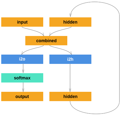
After that, we are going to define a RNN structure like the following:
Considering the output of prediction is merely a number, we need to convert this numerical value into a language category.
The last step before we dive into the training, we have to write a training data sampling function.
Train the Network
We use nn.NLLLoss() (negative log likelihood loss) as loss function and SGD with lr=0.005 as optimizater.
Referneces
The Unreasonable Effectiveness of Recurrent Neural Networks
minimal character-level RNN language model in Python/numpy
Recurrent Neural Networks by Example in Python
Understanding Stateful LSTM Recurrent Neural Networks in Python with Keras