Attention in DP and NLP.
Attention in Seq2seq
Remember that our seq2seq model is made of two parts, an encoder that encodes the input sentence, and a decoder that leverages the information extracted by the decoder to produce the translated sentence. Basically, our input is a sequence of words $x_1, …, x_n$ that we want to translate, and our target sentecne is a sequence of words $y_1,…,y_m$.
Encoder
Let $(h_1,…,h_n)$ be the hidden vectors representing the input sentence. These vectors are the output of a bi-LSTM for instance, and capture contextual representation of each word in the sentence.
Decoder
We want to computer the hidden states $s_i$ of the decoder using a recursive formula of the form
where $s_{i-1}$ is the previous hidden vector, $y_{i-1}$ is the generated word at the previous step, and $c_i$ is a context vector that capture the context from the original sentence that is relevant to the time step $i$ of the decoder.
The contect vector $c_i$ captures relevant information for the $i$-th decoding time step. For each hidden vector from the original sentence $h_j$, compute a score
where a is any function with values in $R$, for instance a single layer fully-connceted neural network. Then, we end up with a scalar vaules $e_{i,1},…,e_{i,n}$. Normalize these scores into a vector $\alpha_i=(\alpha_{i,1},…,\alpha_{i,n})$, using a softmax layer.
Then, compute the context vector $c_i$ as the weighted average of the hidden vectors from the original sentence
Intuitively, this vector captures the relevant contextual information from the original sentence for the $i$-th step of the decoder.
Attention in General
In essence, I will describe Attention Parameters as a projection of a query for a series of key-value pairs as in the below image:
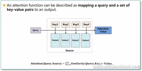
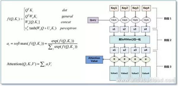
Calculating attention comes primarily in three steps. First, we take the query and each key and compute the similarity between the two to obtain a weight. Frequently used similarity functions include dot product, splice, detector, etc. The second step is typically to use a softmax function to normalize these weights, and finally to weight these weights in conjunction with the corresponding values and obtain the final Attention.
In current NLP work, the key and value are frequently the same, therefore key=value.
Self-Attention
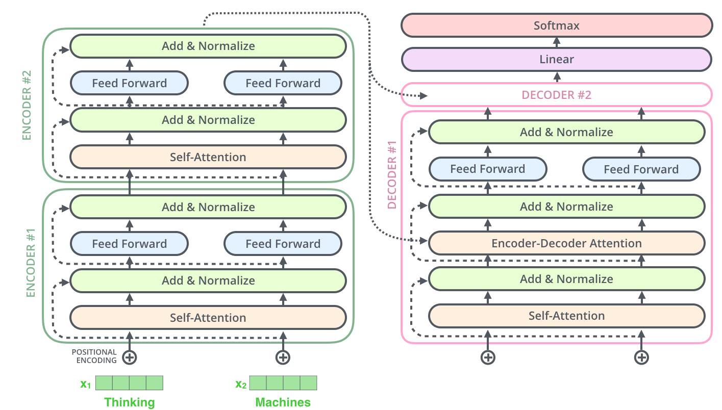
The encoding component is a stack of encoders (the paper stacks six of them on top of each other – there’s nothing magical about the number six, one can definitely experiment with other arrangements). The decoding component is a stack of decoders of the same number.
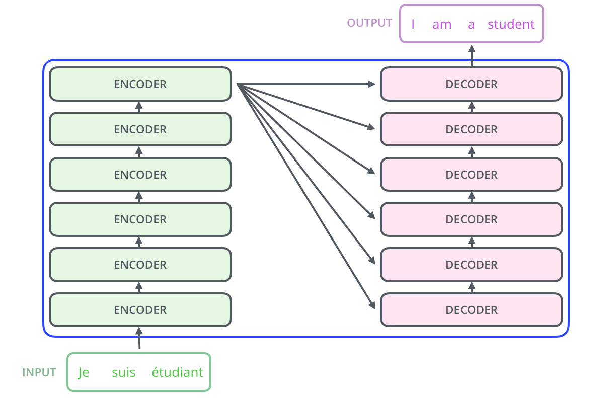
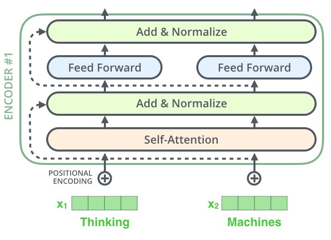
The encoders are all identical in structure (yet they do not share weights). Each one is broken down into two sub-layers:
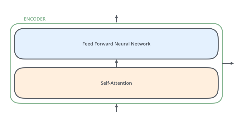 The encoder’s input first flow through a self-attention layer – a layer that helps the encoder look at other words in the input sentence as it encodes a specific word. The outputs of the self-attention layer are fed to a feed-forward neural network. The decoder has both those layers, but between them is an attention layer that helps the decoder focus on relevant parts of the input sentence.

In decoder, the target is fed into the self-attention layer. And the outputs from this layer and encoder are sent to encoder-decoder attention layer.
Bring the tensors into the picture
Now that we’ve seen the major components of the model, let’s start to look at the various vectors/tensors and how they flow between these components to turn the input of a trained model into an output.
As is the case in NLP applications in general, we begin by turning each input word into a vector using an embedding layer.

After embedding the words in our input sequence, each of them flows through each of the two layers of the encoder.
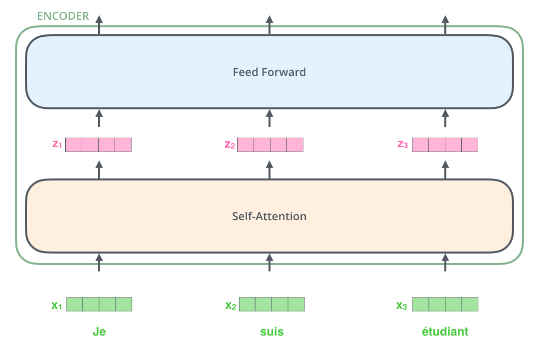
The first step in calculating self-attention is to create three vectors from each of the encoder’s input vectors (in this case, the embedding of each word). So for each word, we create a Query vector, a Key vector, and a Value vector. These vectors are created by multiplying the embedding by three matrices that we trained during the training process.
Notice that these new vectors are smaller in dimension than the embedding vector. Their dimensionality is 64, while the embedding and encoder input/output vectors have dimensionality of 512. They don’t HAVE to be smaller, this is an architecture choice to make the computation of multiheaded attention (mostly) constant.
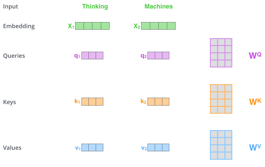
The second step in calculating self-attention is to calculate a score. Say we’re calculating the self-attention for the first word in this example, “Thinking”. We need to score each word of the input sentence against this word. The score determines how much focus to place on other parts of the input sentence as we encode a word at a certain position.
The score is calculated by taking the dot product of the query vector with the key vector of the respective word we’re scoring. So if we’re processing the self-attention for the word in position #1, the first score would be the dot product of q1 and k1. The second score would be the dot product of q1 and k2.
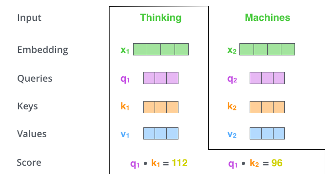
The third and forth steps are to divide the scores by 8 (the square root of the dimension of the key vectors used in the paper – 64. This leads to having more stable gradients. There could be other possible values here, but this is the default), then pass the result through a softmax operation. Softmax normalizes the scores so they’re all positive and add up to 1.
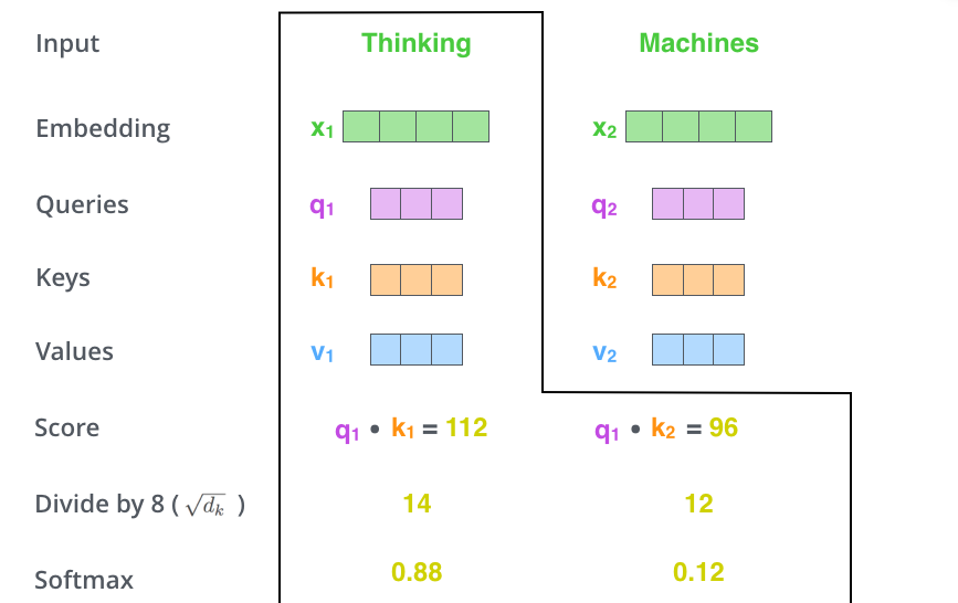
This softmax score determines how much how much each word will be expressed at this position. Clearly the word at this position will have the highest softmax score, but sometimes it’s useful to attend to another word that is relevant to the current word.
The fifth step is to multiply each value vector by the softmax score (in preparation to sum them up). The intuition here is to keep intact the values of the word(s) we want to focus on, and drown-out irrelevant words (by multiplying them by tiny numbers like 0.001, for example).
The sixth step is to sum up the weighted value vectors. This produces the output of the self-attention layer at this position (for the first word).
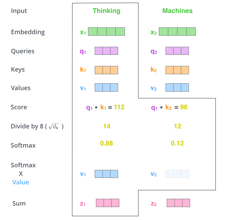
That concludes the self-attention calculation. The resulting vector is one we can send along to the feed-forward neural network. In the actual implementation, however, this calculation is done in matrix form for faster processing. So let’s look at that now that we’ve seen the intuition of the calculation on the word level.
Matrix calculation of Self-Attention
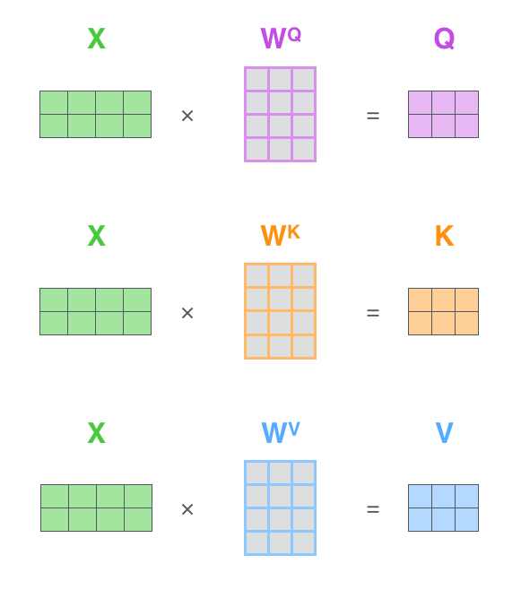
The first step is to calculate the Query, Key, and Value matrices. We do that by packing our embeddings into a matrix X, and multiplying it by the weight matrices we’ve trained (WQ, WK, WV).
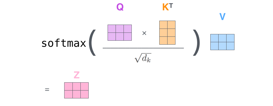
Finally, since we’re dealing with matrices, we can condense steps two through six in one formula to calculate the outputs of the self-attention layer.
Multi heads
The paper further refined the self-attention layer by adding a mechanism called “multi-headed” attention. This improves the performance of the attention layer in two ways:
- It expands the model’s ability to focus on different positions. Yes, in the example above, z1 contains a little bit of every other encoding, but it could be dominated by the the actual word itself. It would be useful if we’re translating a sentence like “The animal didn’t cross the street because it was too tired”, we would want to know which word “it” refers to.
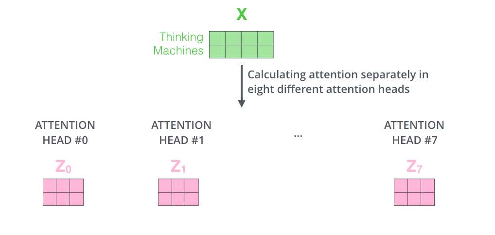
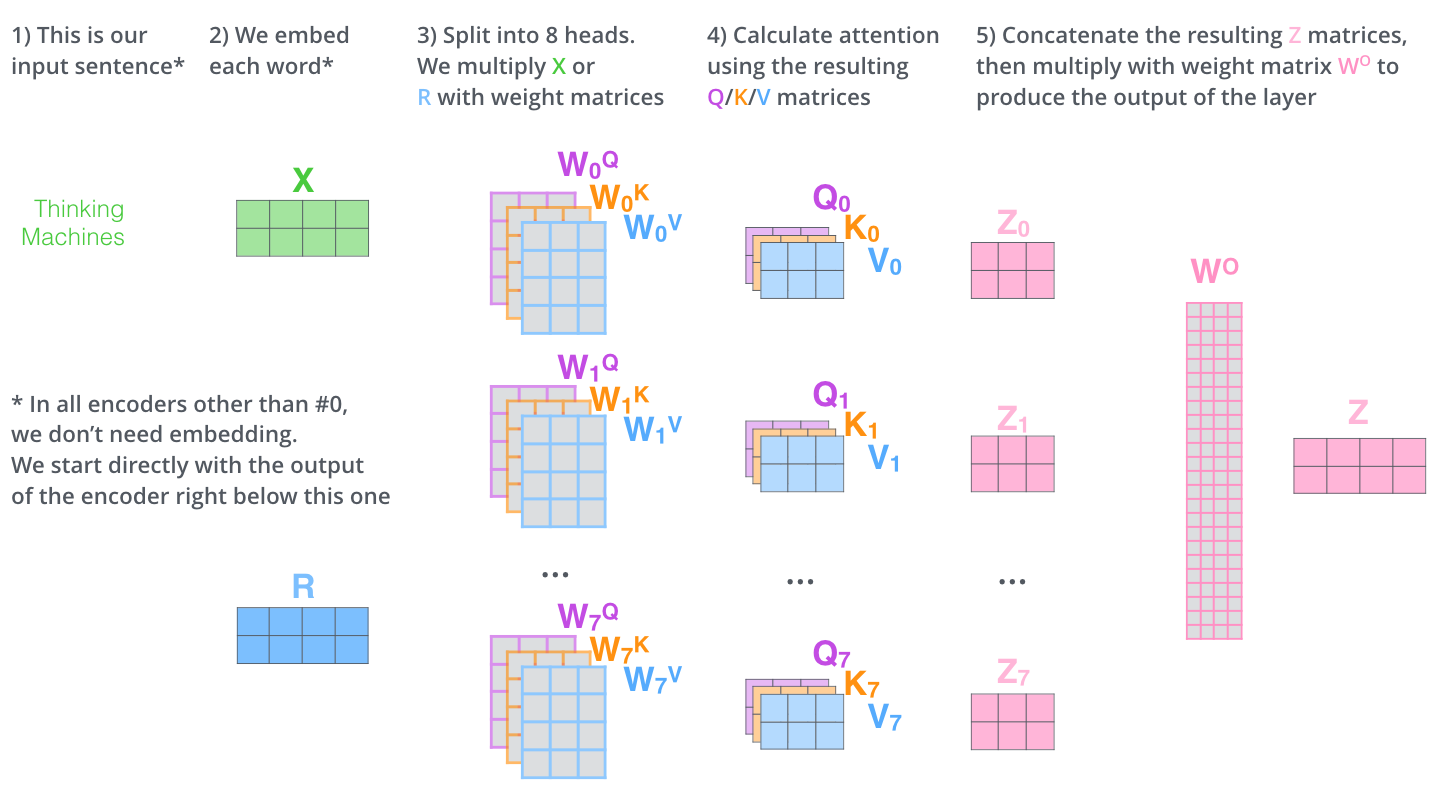
- It gives the attention layer multiple “representation subspaces”. As we’ll see next, with multi-headed attention we have not only one, but multiple sets of Query/Key/Value weight matrices (the Transformer uses eight attention heads, so we end up with eight sets for each encoder/decoder). Each of these sets is randomly initialized. Then, after training, each set is used to project the input embeddings (or vectors from lower encoders/decoders) into a different representation subspace.
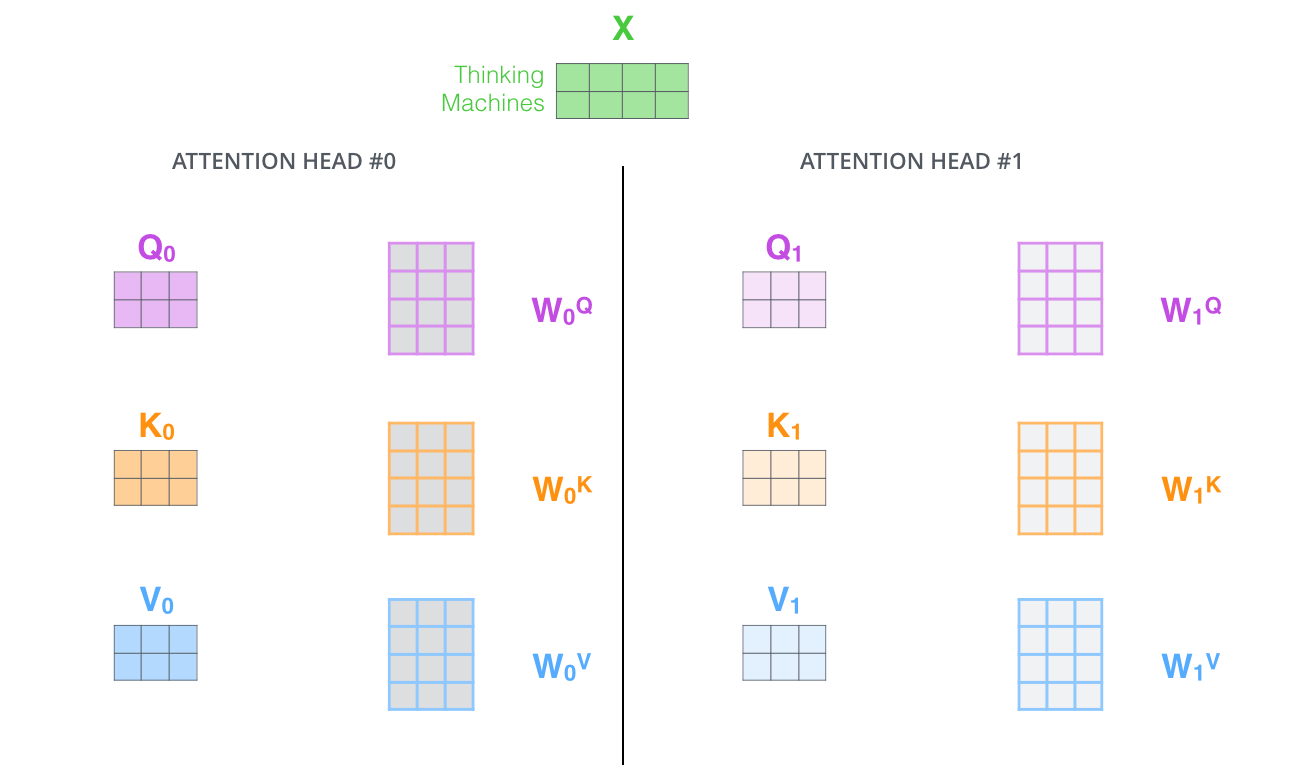
If we do the same self-attention calculation we outlined above, just eight different times with different weight matrices, we end up with eight different Z matrices
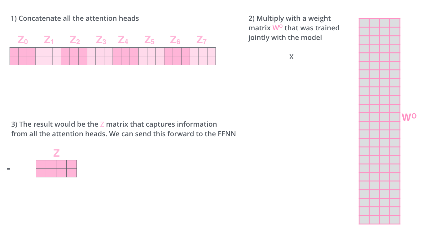
We concat the matrices then multiple them by an additional weights matrix WO.
That’s pretty much all there is to multi-headed self-attention. It’s quite a handful of matrices, I realize. Let me try to put them all in one visual so we can look at them in one place
Sequence order
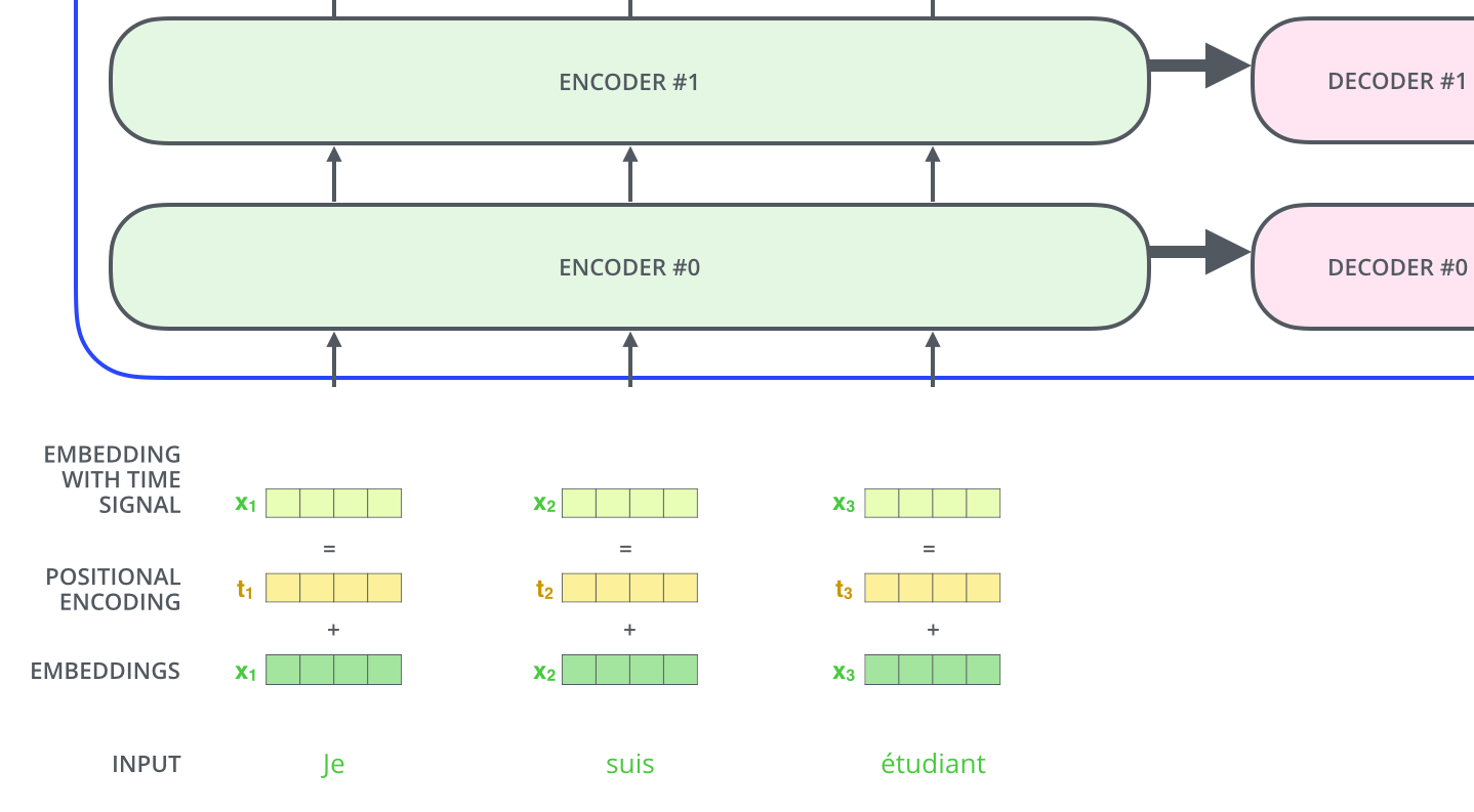
One thing that’s missing from the model as we have described it so far is a way to account for the order of the words in the input sequence.
To address this, the transformer adds a vector to each input embedding. These vectors follow a specific pattern that the model learns, which helps it determine the position of each word, or the distance between different words in the sequence. The intuition here is that adding these values to the embeddings provides meaningful distances between the embedding vectors once they’re projected into Q/K/V vectors and during dot-product attention.
The residuals
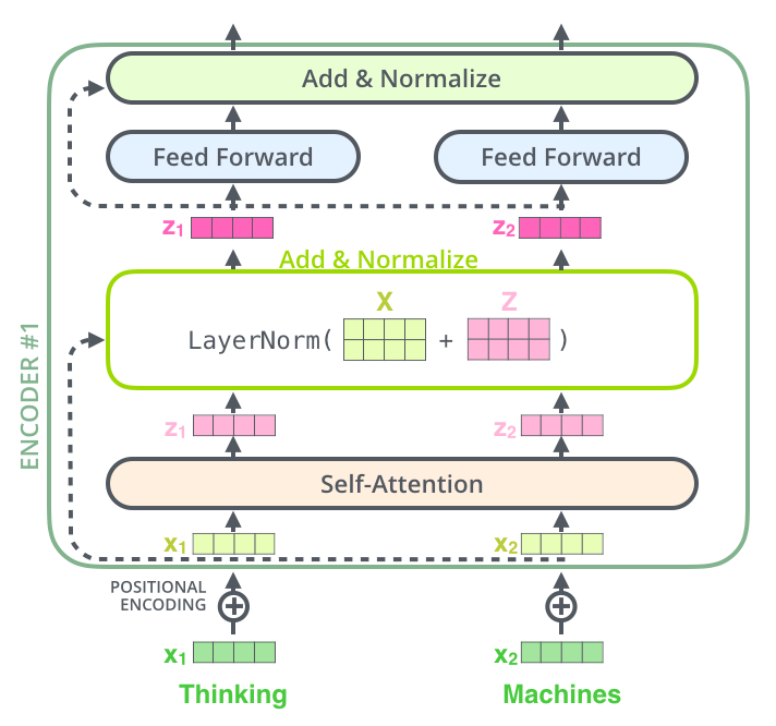
One detail in the architecture of the encoder that we need to mention before moving on, is that each sub-layer (self-attention, ffnn) in each encoder has a residual connection around it, and is followed by a layer-normalization step.
If we’re to visualize the vectors and the layer-norm operation associated with self attention, it would look like this:
This goes for the sub-layers of the decoder as well. If we’re to think of a Transformer of 2 stacked encoders and decoders, it would look something like this:
Decoder side
The encoder start by processing the input sequence. The output of the top encoder is then transformed into a set of attention vectors K and V. These are to be used by each decoder in its “encoder-decoder attention” layer which helps the decoder focus on appropriate places in the input sequence
The following steps repeat the process until a special symbol is reached indicating the transformer decoder has completed its output. The output of each step is fed to the bottom decoder in the next time step, and the decoders bubble up their decoding results just like the encoders did. And just like we did with the encoder inputs, we embed and add positional encoding to those decoder inputs to indicate the position of each word.
The self attention layers in the decoder operate in a slightly different way than the one in the encoder:
In the decoder, the self-attention layer is only allowed to attend to earlier positions in the output sequence. This is done by masking future positions (setting them to -inf) before the softmax step in the self-attention calculation.
The “Encoder-Decoder Attention” layer works just like multiheaded self-attention, except it creates its Queries matrix from the layer below it, and takes the Keys and Values matrix from the output of the encoder stack.
Attention in GAN
Convolutional GANs have difficulty in learning the image distributions of diverse multi-class datasets like Imagenet. It is observed that CGANs could easily generate images with a simpler geometry like Ocean, Sky etc. but failed on images with some specific geometry like dogs, horses and many more.
This problem is arising because the convolution is a local operation whose receptive field depends on the spatial size of the kernel. In a convolution operation, it is not possible for an output on the top-left position to have any relation to the output at bottom-right.
You would ask, Can’t we make the spatial size bigger so that it captures more of the image? Yes! of course we can, but it would decrease computational efficiency achieved by smaller filters and make the operation slow. Then you would again ask, Can’t we make a Deep CGAN with smaller filters so that the later layers have a large receptive field? Yes! we can, but it would take too many layers to have a large enough receptive field and too many layers would mean too many parameters. Hence it would make the GAN training more unstable.
The solutions to keeping computational efficiency and having a large receptive field at the same time is Self-Attention. It helps create a balance between efficiency and long-range dependencies(= large receptive fields) by utilizing the famous mechanism from NLP called attention.
The model
The work process is as follows
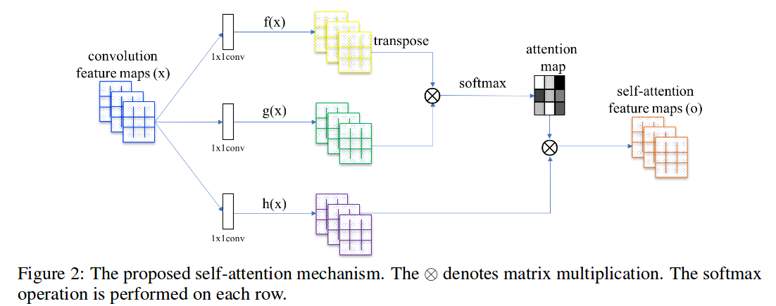
On the left of the below image, we get our feature maps from the previous convolutional layer. Let’s suppose it is of the dimension $(512\times 7 \times 7)$ where 512 is the number of channels and 7 is the spatial dimension. We first pass the feature map through three $1\times 1$ convolutions separately. We name the three filters $f, g$ and $h$.
What $1\times 1$ convolution does is that it reduces the channel number in the image. The filter size of $f$ and $g$ is 64 while the size of $h$ is 512. After the image gets passed through we get three feature maps of dimensions $(64\times 7\times 7)$, $(64\times 7\times 7)$ and $(512\times 7\times 7)$. These three things are our query, key and value pairs. In order to perform self attention onthe complete image, we flatten out last two dimensions and the dimensions become $(64\times 49)$, $(64\times 49)$, $(512\times 49)$. We transpose the query and matrix-multiply it by the key and take the softmax on all the rows. So we get an output attention map of shape $(49\times 49)$. Then we multiple the value vector with the attention map, resulting in output with $(512\times 49)$. One last thing that the paper proposes is that to multiply the final output by a learnable scale parameter and add back the input as a residual connection. Let’s say the $x$ is the image and $o$ is the output, we multiple $o$ by a parameter $y$. The final output $O$ is $O=yo+x$. Initially, the paper advises initializing the sacle parameter as zero so that the output is simple old convolution at the beginning. They initialized $y$ with zero because they wanted their network to rely on the cues in the local neighborhood — since that was easier and then gradually the network will learn to assign the value to y* parameter and use self-attention.
Language Model
Language modeling is the task of predicting what word comes next. More formally, given a sequence of words $x^{(1)}, x^{(2)},…,x^{(t)}, $ compute the probability distribution of the next word $x^{(t+1)}$:
where $x^{t+1}$ can be any word in the vocabulary $V={w_1,…,w_{|V|}}$. A system that does this is called a Language Model.
We can also think of a Language Model as a system that assigns probability to a piece of text. For example, if we have some text $x^{(1)}, x^{(2)},…,x^{(T)}$, then the probability of this text is:
N-gram Language Models
Definition: A n-gram is a chunk of n consecutive words.
Idea: Collect statistics about how frequent different n-grams are, and use these to predict next word.
Assumption: $x^{t=1}$ depends only on the preceding $n-1$ words.
Counting: by counting in some large corpus of text, we get these n-gram and (n-1)-gram probabilities.
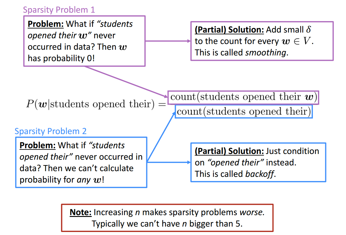
Problems:
Sparsity Problems with n-gram Language Models
Storage Problems with n-gram Language Models
Need to store count for all n-grams you saw in the corpus and increasing n or increasing corpus increases model size!
Neural Language Model
A fixed-window neural Language Model
Say we have the sentence:

Then we use the neural network to build the model
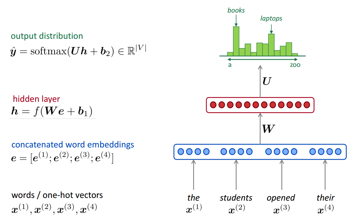
Improvements over n-gram LM:
- No sparsity problem
- Don’t need to store all observed n-grams
Remaining problems:
- Fixed window is too small
- Enlarging window enlarges $W$ while Window can never be large enough!
- $ x^{(1)}$and $ x^{(2)}$ are multiplied by completely different weights in $W$. No symmetry in how the inputs are processed.
We need a neural architecture that can process any length input.
RNN
Core idea: Apply the same weights $W$ repeatedly.
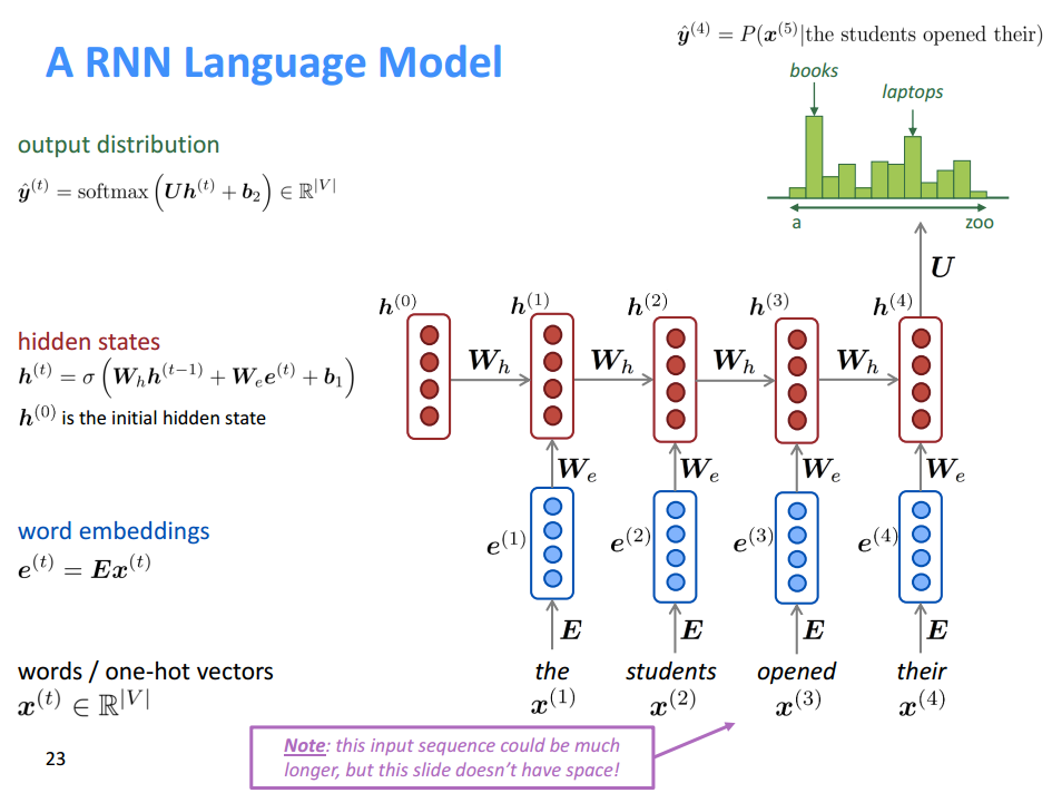
RNN Advantages:
- Can process any length input
- Computation for step t can (in theory) use information from many steps back
- Model size doesn’t increase for longer input
- Same weights applied on every timestep, so there is symmetry in how inputs are processed.
RNN Disadvantages:
- Recurrent computation is slow
- In practice, difficult to access information from many steps back
Training a RNN
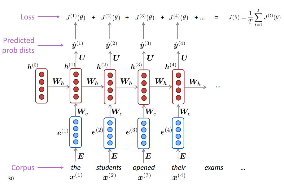
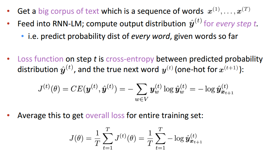
Evaluating Language Models
In general, perplexity is a measurement of how well a probability model predicts a sample.
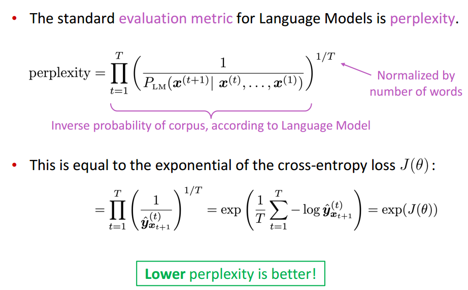
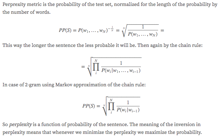
Normalizing by the length is to avoid the pitfall that bigger corpus have smaller perplexity.