DP-FullyConvolutionalSegmentation

This post is based on the paper Fully Convolutional Networks for Semantic Segmentation, which aims to perform image segmentation.

Overview

ref

More specifically, the goal of semantic image segmentation is to label each pixel of an image with a corresponding class of what is being represented. Because we’re predicting for every pixel in the image, this task is commonly referred to as dense prediction.

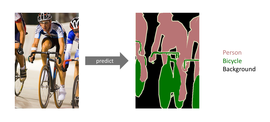
One important thing to note is that we’re not separating instances of the same class; we only care about the category of each pixel. In other words, if you have two objects of the same category in your input image, the segmentation map does not inherently distinguish these as separate objects. There exists a different class of models, known as instance segmentation models, which do distinguish between separate objects of the same class.

Segmentation models are useful for a variety of tasks, including:

• Autonomous vehicles
  We need to equip cars with the necessary perception to understand their environment so that self-driving cars can safely integrate into our existing roads.

  

• Medical image diagnostics

Representing the task

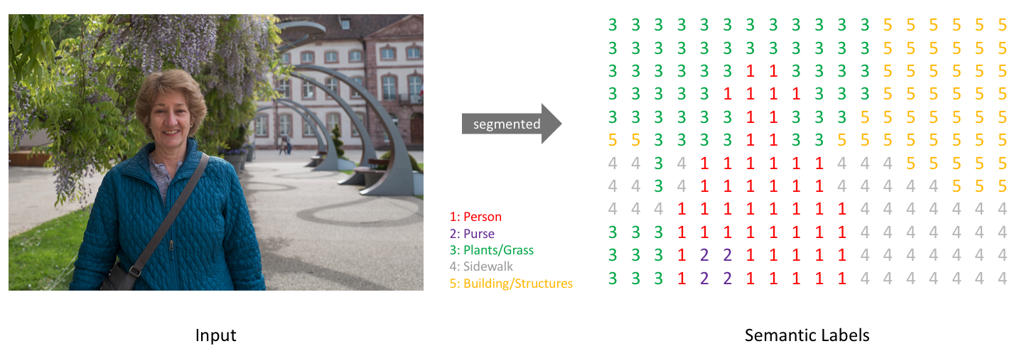
Simply, our goal is to take either a RGB color image (height×width×3height×width×3) or a grayscale image (height×width×1height×width×1) and output a segmentation map where each pixel contains a class label represented as an integer (height×width×1height×width×1).

Similar to how we treat standard categorical values, we’ll create our target by one-hot encoding the class labels - essentially creating an output channel for each of the possible classes.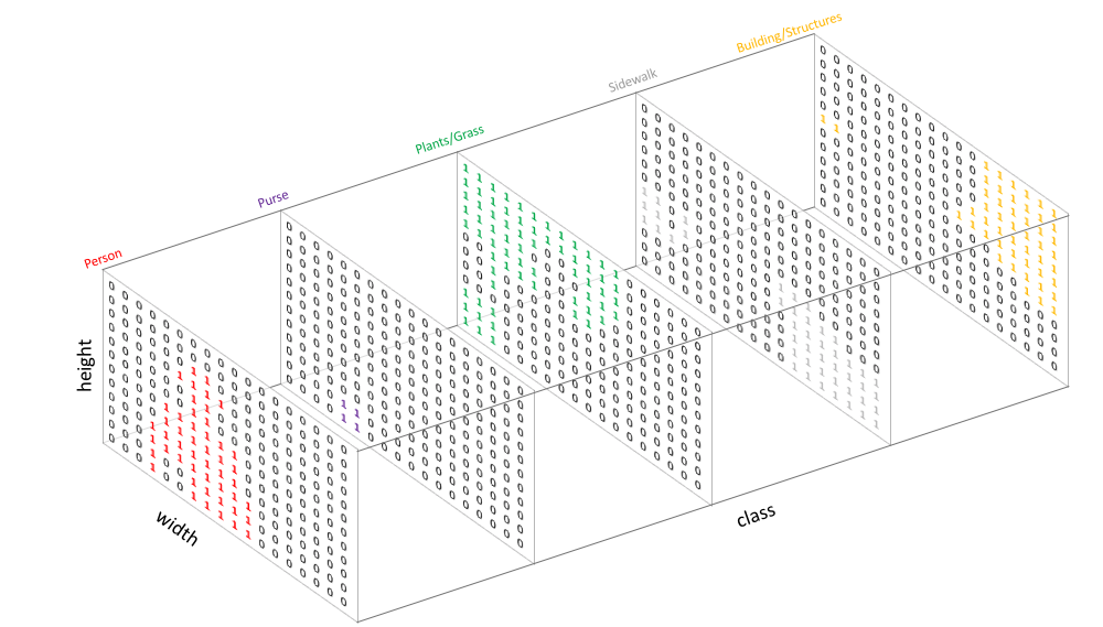

A prediction can be collapsed into a segmentation map (as shown in the first image) by taking the argmax of each depth-wise pixel vector.

Fully convolutional networks

In the traditional image classification deep learning architecture, we take a image and pass this image through a number of convolution layers so that we get the high-level features. And the features are connected with several dense layers and output the classification prediction.

In FCN, image segmentation models is to follow an encoder/decoder structure where we downsample the spatial resolution of the input, developing lower-resolution feature mappings which are learned to be highly efficient at discriminating between classes, and the upsample the feature representations into a full-resolution segmentation map.

Upsampling ref

There are a few different approaches that we can use to upsample the resolution of a feature map.

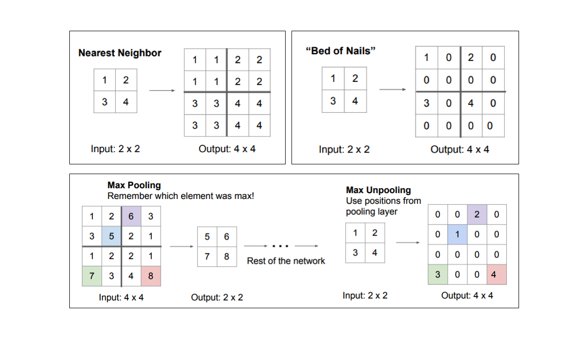
However, transpose convolutions are by far the most popular approach as they allow for us to develop a learned upsampling.

Before diving into transpose convolutions, we review what convolutions do. Suppose We are applying the convolution to an image of 5x5x1 with a kernel of 3x3, stride 2x2 and padding VALID.

As you can see in the left image the output will be a 2x2 image. You can calculate the output size of a convolution operation by using below formula as well:

Convolution Output Size = 1 + (Input Size - Filter size + 2 * Padding) / Stride

Now suppose you want to up-sample this to same dimension as input image. You will use same parameters as for convolution and will first calculate what was the size of Image before down-sampling.

SAME PADDING:
Transpose Convolution Size = Input Size Stride
VALID PADDING: 0Transpose Convolution Size = Input Size Stride + max(Filter Size - Stride, 0)

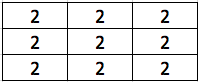
Suppose we have the following image:

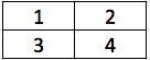
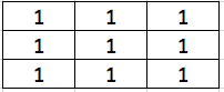
For transpose convolution, we use $3 \times 3$ filter and stride 2, then we go over each pixel and each single pixel is multiplied by a $3\times 3$ filter and formed a $3 \times 3$ block which is then put in output matrix. Say the initial filter is all-one matrix, so after processing the first pixel, we have:

For the second pixel, we have:

Since the stride step is 2, so we are going to combine the above two matrix:

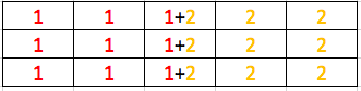
we get $3 \times 5$ matrix.

For the third and fouth matrix, we have

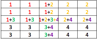
So after the deconvolution, we have $5\times 5$ matrix:

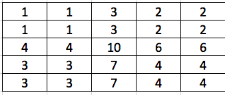
To sum up, the convolution transpose is the opposite of convolution. Since for convolution, the new size is (old_row - k + 2*p ) / s + 1, so for convolution transpose, its size is (old_row - 1) * s - 2*p + k. If we use no padding and kernel size equals stride step, then new size is old_row * s.

Network Structures

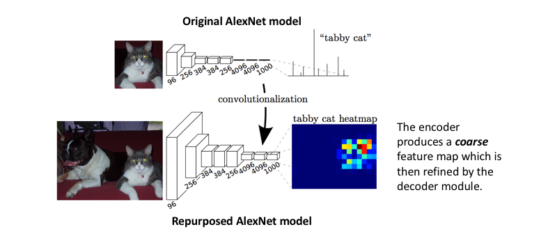
The original paper use well-studied image classification networks (eg. AlexNet) to serve as the encoder module of the network, appending a decoder module with transpose convolutional layers to upsample the coarse feature maps into a full-resolution segmentation map. The encoder structure looks like the following:

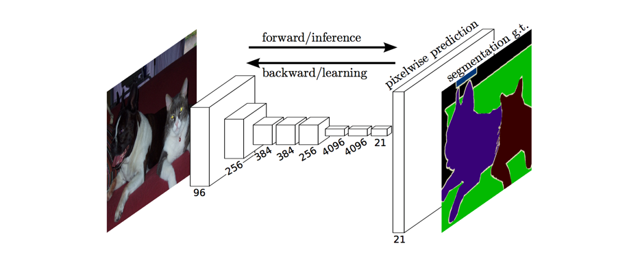
The full network, as shown below, is trained according to a pixel-wise cross entropy loss.

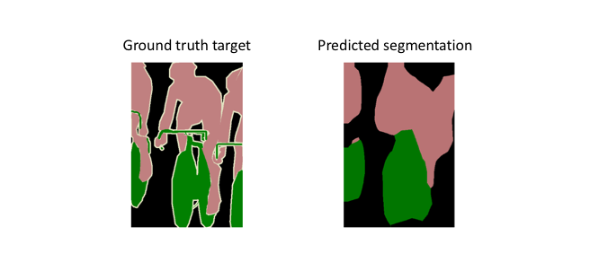
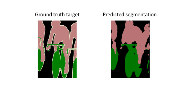
However, because the encoder module reduces the resolution of the input by a factor of 32, the decoder module struggles to produce fine-grained segmentations (as shown below).

The paper’s authors comment eloquently on this struggle:

Semantic segmentation faces an inherent tension between semantics and location: global information resolves what while local information resolves where… Combining fine layers and coarse layers lets the model make local predictions that respect global structure. ― Long et al.

Skip Connections

The authors address this tension by slowly upsampling (in stages) the encoded representation, adding “skip connections” from earlier layers, and summing these two feature maps.

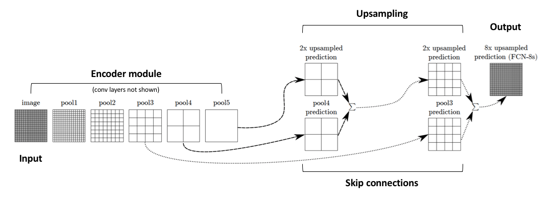
These skip connections from earlier layers in the network (prior to a downsampling operation) should provide the necessary detail in order to reconstruct accurate shapes for segmentation boundaries. Indeed, we can recover more fine-grain detail with the addition of these skip connections.

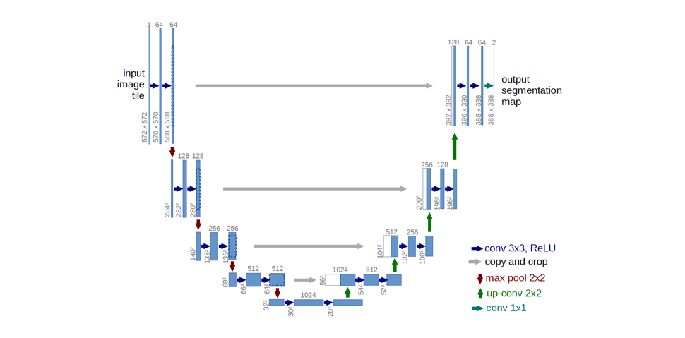
Ronneberger et al. improve upon the “fully convolutional” architecture primarily through expanding the capacity of the decoder module of the network. More concretely, they propose the U-Net architecture which “consists of a contracting path to capture context and a symmetric expanding path that enables precise localization.” This simpler architecture has grown to be very popular and has been adapted for a variety of segmentation problems.

Loss function

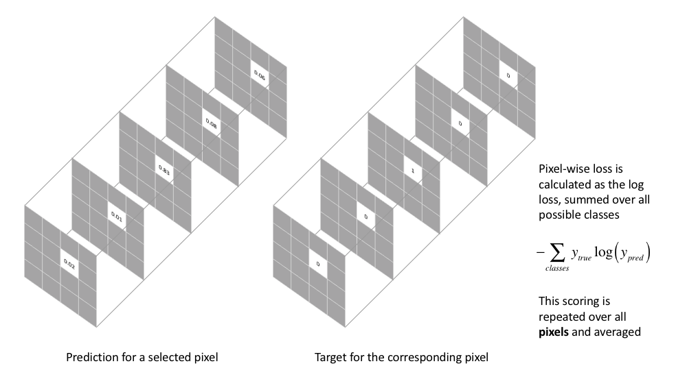
The most commonly used loss function for the task of image segmentation is a pixel-wise cross entropy loss. This loss examines each pixel individually, comparing the class predictions (depth-wise pixel vector) to our one-hot encoded target vector.

Because the cross entropy loss evaluates the class predictions for each pixel vector individually and then averages over all pixels, we’re essentially asserting equal learning to each pixel in the image. This can be a problem if your various classes have unbalanced representation in the image, as training can be dominated by the most prevalent class. Long et al. (FCN paper) discuss weighting this loss for each output channel in order to counteract a class imbalance present in the dataset.

Implementation

In order to get a full understanding of FCN, we will get our hands on streetview images segmentation. The state of the art dataset is pascal VOC2012, however it requires preprocessing and is kind of large, we choose a streetview dataset with 12 object classes which includes 367 training dataset and 101 test images. It is perfect for us to feel how FCN works in image segmentation.

Data exploration

The data directory looks like the following:

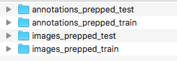
where in the images_prepped_train there are original images for training, while in annotations_prepped_train is our groundtruth for each image. For a groundtruth image, it is the same size with the original image where each pixel is labeled with a class. It is same with the test images directory.

The first thing to do is to visualize a single segmentation image.

import cv2,os
import numpy as np
import matplotlib.pyplot as plt
import seaborn as sns

dir_seg = "/Users/daniel/Desktop/streets/annotations_prepped_train/"
dir_img = "/Users/daniel/Desktop/streets/images_prepped_train/"

n_classes = 12 #total classes for segmentation

ldseg = os.listdir(dir_seg)
firstimage = ldseg[0] # choose the first image for visualization

seg = cv2.imread(dir_seg+firstimage) # read segmentation groundtruth
img = cv2.imread(dir_img+firstimage) # read original image

mi,ma = np.min(seg),np.max(seg) #get the range for classes
total_classes = ma-mi+1 
# print("The total segmentation classes are : {}".format(ma-mi+1))

fig = plt.figure(figsize=(5,5))
ax = fig.add_subplot(1,1,1)
ax.imshow(img)
ax.set_title("Original Image")

fig = plt.figure(figsize=(15,10))
for k in range(mi,ma+1):
    ax = fig.add_subplot(3,total_classes/3,k+1) #the first digit is the number of rows, the second the number of columns, and the third the index of the subplot.
    ax.imshow((seg==k)*1.0) #(seg==k) return a True/False list
    ax.set_title("label={}".format(k))
plt.show()

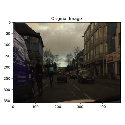
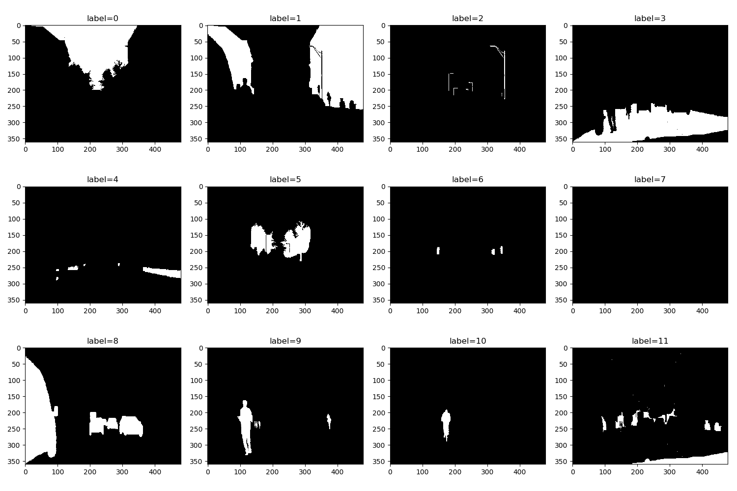
We can roughly observe from the segmentaion image that the first class is buildings, while the class label=8 is cars.

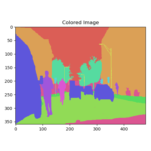
Next, I will give the different objects with different colors to visualize them in one image.

def img_colorized(seg,n_classes):
    if len(seg.shape) == 3:
        seg = seg[:, :, 0]
    seg_img = np.zeros((seg.shape[0], seg.shape[1], 3)).astype('float')
    colors = sns.color_palette("hls", n_classes) # return n_classes colors

    for c in range(n_classes):
        segc = (seg == c)
        seg_img[:, :, 0] += (segc * (colors[c][0]))
        seg_img[:, :, 1] += (segc * (colors[c][1]))
        seg_img[:, :, 2] += (segc * (colors[c][2]))

    return (seg_img)

color_img = img_colorized(seg,n_classes)
fig = plt.figure(figsize=(5,5))
ax = fig.add_subplot(1,1,1)
ax.imshow(color_img)
ax.set_title("Colored Image")
plt.show()

Data preprocessing

We will resize the image to (224,224). In the following code, we resize the image and normalize the image to range (-1,1).

def dataProcessing(path,width,height):
    img = cv2.imread(path,1)
    img = np.float32(cv2.resize(img,(width,height)))/127.5-1
    return img

Then considering we are going to predict class label for each pixel, so for each pixel, there are going to be total_classes output. So for a input image with size (row,col), the output should be (row, col, total_classes). Therefore, for each groundtruth image, we are going to generate total_classes groundtruth lable images, where in the first image, the pixel belonging to class 0 has value 1 while the rest has value 0.

def getSegmentationArr(path,nClasses,width,height):
    seg_labels = np.zeros((height,width,nClasses))
    img = cv2.imread(path,1)
    img = cv2.resize(img,(width,height))
    img = img[:,:,0]
    for c in range(nClasses):
        seg_labels[:, :, c] = (img == c).astype(int)
    return seg_labels

Then we create our training dataset:

images = os.listdir(dir_img)
images.sort()
segmentations = os.listdir(dir_seg)
segmentations.sort()

X = []
Y = []
for im, seg in zip(images, segmentations):
    X.append(dataProcessing(dir_img + im, 224, 224))
    Y.append(getSegmentationArr(dir_seg + seg, total_classes, 224, 224))

X, Y = np.array(X), np.array(Y)

Network architecture

Then we can implement the network, here we use the vgg16 architecture, where the architecture looks like:

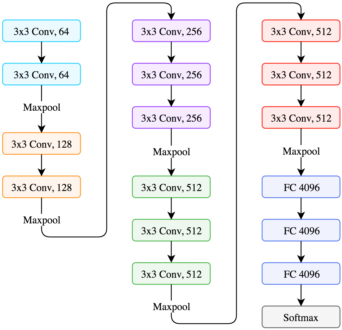
Since the vgg16 downsample the input image to the original size of $1/2^5=1/32$ due to maxpooling. Therefore we need to ensure the input size can be divided by 32. In the beginning, we implement the structure of vgg16: block1 -> block2 -> block3 -> block4 -> block5 .

In order to keep more information, we directly use output from block3 and block4 to combine them with the output of block5. To be specific, for the output of block5, we use conv2d_k4096_s7 + conv2d_k4096_s1 + conv2dT_k12_s4_p4; for the output of block4, we need to upsample it by 2, conv2d_k12_s1 + conv2dT_k12_s2_p2; for output of block3, conv2d_k12_s1. And finally, combine them by adding them.

from keras.models import *
from keras.layers import *
warnings.filterwarnings("ignore")

vgg_weights = 'vgg16_weights_tf_dim_ordering_tf_kernels_notop.h5'

def FCN8(nClasses,input_height=224,input_width=224):
    assert  input_height%32 == 0
    assert input_width%32 == 0

    img_input = Input(shape=(input_height, input_width, 3))  ## Assume 224,224,3

    ## Block 1
    x = Conv2D(64, (3, 3), activation='relu', padding='same', name='block1_conv1')(
        img_input)
    x = Conv2D(64, (3, 3), activation='relu', padding='same', name='block1_conv2')(x)
    x = MaxPooling2D((2, 2), strides=(2, 2), name='block1_pool')(x)
    f1 = x

    # Block 2
    x = Conv2D(128, (3, 3), activation='relu', padding='same', name='block2_conv1')(x)
    x = Conv2D(128, (3, 3), activation='relu', padding='same', name='block2_conv2')(x)
    x = MaxPooling2D((2, 2), strides=(2, 2), name='block2_pool')(x)
    f2 = x

    # Block 3
    x = Conv2D(256, (3, 3), activation='relu', padding='same', name='block3_conv1')(x)
    x = Conv2D(256, (3, 3), activation='relu', padding='same', name='block3_conv2')(x)
    x = Conv2D(256, (3, 3), activation='relu', padding='same', name='block3_conv3')(x)
    x = MaxPooling2D((2, 2), strides=(2, 2), name='block3_pool')(x)
    pool3 = x

    # Block 4
    x = Conv2D(512, (3, 3), activation='relu', padding='same', name='block4_conv1')(x)
    x = Conv2D(512, (3, 3), activation='relu', padding='same', name='block4_conv2')(x)
    x = Conv2D(512, (3, 3), activation='relu', padding='same', name='block4_conv3')(x)
    pool4 = MaxPooling2D((2, 2), strides=(2, 2), name='block4_pool')(x)  ## (None, 14, 14, 512)

    # Block 5
    x = Conv2D(512, (3, 3), activation='relu', padding='same', name='block5_conv1')(pool4)
    x = Conv2D(512, (3, 3), activation='relu', padding='same', name='block5_conv2')(x)
    x = Conv2D(512, (3, 3), activation='relu', padding='same', name='block5_conv3')(x)
    pool5 = MaxPooling2D((2, 2), strides=(2, 2), name='block5_pool')(x)  ## (None, 7, 7, 512)

    vgg = Model(img_input, pool5)
    vgg.load_weights(vgg_weights)  ## loading VGG weights for the encoder parts of FCN8
#########################################################
    n = 4096
    o = Conv2D(n, (7, 7), activation='relu', padding='same', name="conv6")(pool5)
    conv7 = Conv2D(n, (1, 1), activation='relu', padding='same', name="conv7")(o)

    ## 4 times upsamping for pool4 layer
    conv7_4 = Conv2DTranspose(nClasses, kernel_size=(4, 4), strides=(4, 4), use_bias=False)(conv7)
    ## (None, 224, 224, 10)
    ## 2 times upsampling for pool411
    pool411 = Conv2D(nClasses, (1, 1), activation='relu', padding='same', name="pool4_11")(pool4)
    pool411_2 =Conv2DTranspose(nClasses, kernel_size=(2, 2), strides=(2, 2), use_bias=False)(pool411)

    pool311 = Conv2D(nClasses, (1, 1), activation='relu', padding='same', name="pool3_11")(pool3)

    o = Add(name="add")([pool411_2, pool311, conv7_4])
    o = Conv2DTranspose(nClasses, kernel_size=(8, 8), strides=(8, 8), use_bias=False)(o)
    o = Activation('softmax')(o)

    model = Model(img_input, o)

    return model

model = FCN8(nClasses=n_classes,input_height=224,input_width=224)
model.summary()

Training

from sklearn.utils import shuffle
train_rate = 0.85
index_train = np.random.choice(X.shape[0],int(X.shape[0]*train_rate),replace=False)
index_test  = list(set(range(X.shape[0])) - set(index_train))
X, Y = shuffle(X,Y)
X_train, y_train = X[index_train],Y[index_train]
X_test, y_test = X[index_test],Y[index_test]

from keras import optimizers
sgd = optimizers.SGD(lr=1e-2,decay=5**(-4),momentum=0.9,nesterov=True)
model.compile(loss='categorical_crossentropy',optimizer=sgd,metrics=['accuracy'])

hist = model.fit(X_train,y_train,validation_data=(X_test,y_test),
                 batch_size=32,epochs=200,verbose=2)
model.save("seg_model.h5")

mean Intersection over Union

Intersection over Union is an evaluation metric used to measure the accuracy of an object detector on a particular dataset. However, Any algorithm that provides predicted bounding boxes as output can be evaluated using IoU.

More formally, in order to apply Intersection over Union to evaluate an (arbitrary) object detector we need:

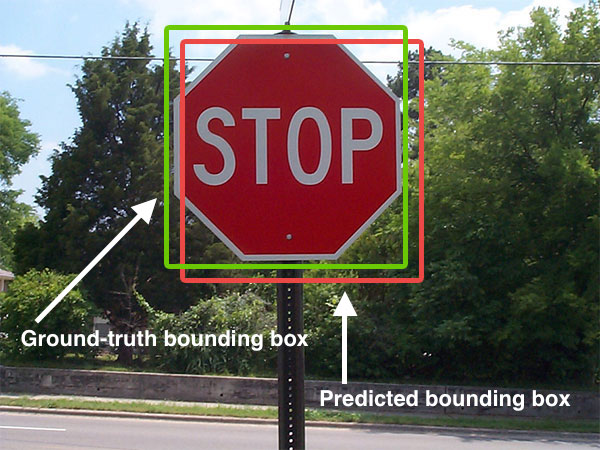
1. The ground-truth bounding boxes (i.e., the hand labeled bounding boxes from the testing set that specify where in the image our object is).
2. The predicted bounding boxes from our model.

As long as we have these two sets of bounding boxes we can apply Intersection over Union.

Below I have included a visual example of a ground-truth bounding box versus a predicted bounding box:

Computing Intersection over Union can therefore be determined via:

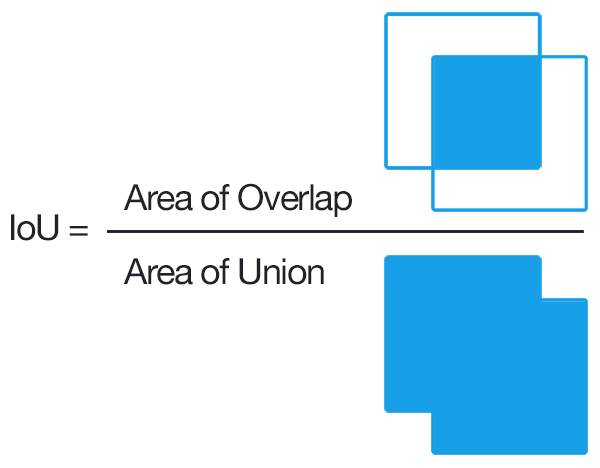
In the numerator we compute the area of overlap between the predicted bounding box and the ground-truth bounding box.

The denominator is the area of union, or more simply, the area encompassed by both the predicted bounding box and the ground-truth bounding box.

def IoU(Yi, y_predi):
    ## mean Intersection over Union
    ## Mean IoU = TP/(FN + TP + FP)

    IoUs = []
    Nclass = int(np.max(Yi)) + 1
    for c in range(Nclass):
        TP = np.sum((Yi == c) & (y_predi == c))
        FP = np.sum((Yi != c) & (y_predi == c))
        FN = np.sum((Yi == c) & (y_predi != c))
        IoU = TP / float(TP + FP + FN)
        print("class {:02.0f}: #TP={:6.0f}, #FP={:6.0f}, #FN={:5.0f}, IoU={:4.3f}".format(c, TP, FP, FN, IoU))
        IoUs.append(IoU)
    mIoU = np.mean(IoUs)
    print("_________________")
    print("Mean IoU: {:4.3f}".format(mIoU))

y_pred = model.predict(X_test)
y_predi = np.argmax(y_pred, axis=3)
y_testi = np.argmax(y_test, axis=3)
IoU(y_testi, y_predi)

WHY WE USE IoU?

In all reality, it’s extremely unlikely that the (x, y)-coordinates of our predicted bounding box are going to exactly match the (x, y)-coordinates of the ground-truth bounding box.

Due to varying parameters of our model (image pyramid scale, sliding window size, feature extraction method, etc.), a complete and total match between predicted and ground-truth bounding boxes is simply unrealistic.

Because of this, we need to define an evaluation metric that rewards predicted bounding boxes for heavily overlapping with the ground-truth.

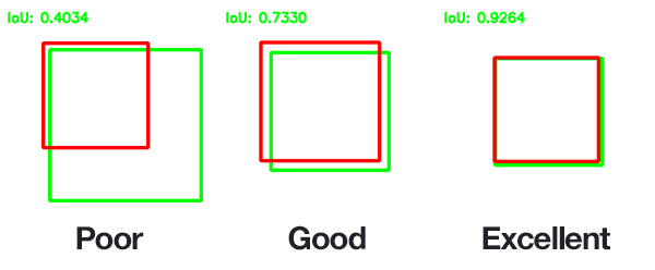
As you can see, predicted bounding boxes that heavily overlap with the ground-truth bounding boxes have higher scores than those with less overlap. This makes Intersection over Union an excellent metric for evaluating custom object detectors.

We aren’t concerned with an exact match of (x, y)-coordinates, but we do want to ensure that our predicted bounding boxes match as closely as possible — Intersection over Union is able to take this into account.

for i in range(10):
    img_is = (X_test[i] + 1) * (255.0 / 2)
    seg = y_predi[i]
    segtest = y_testi[i]

    fig = plt.figure(figsize=(10, 30))
    ax = fig.add_subplot(1, 3, 1)
    ax.imshow(img_is / 255.0)
    ax.set_title("original")

    ax = fig.add_subplot(1, 3, 2)
    ax.imshow(img_colorized(seg, n_classes))
    ax.set_title("predicted class")

    ax = fig.add_subplot(1, 3, 3)
    ax.imshow(img_colorized(segtest, n_classes))
    ax.set_title("true class")
    plt.savefig('{}.png'.format(i))

Conclusion

Overall, in this paper, the most important thing is how use convolution transpose to upsample the feature to the original image size and utilize u-net structure to preserve features for acurate pixel classification. And in the convolution network, we only use convolution and its transpose, that is why it is called Fully Convolution Network.