DP-PyTorch

Tutorials of PyTorch and some useful tips.

Pytorch 101

GPU vs CPU

if torch.cuda.is_available():
    device = torch.device('cuda')
else:
    device = torch.device('cpu')
# Move the data to the proper device (GPU or CPU)
x = x.to(device=device, dtype=dtype)
y = y.to(device=device, dtype=torch.long)
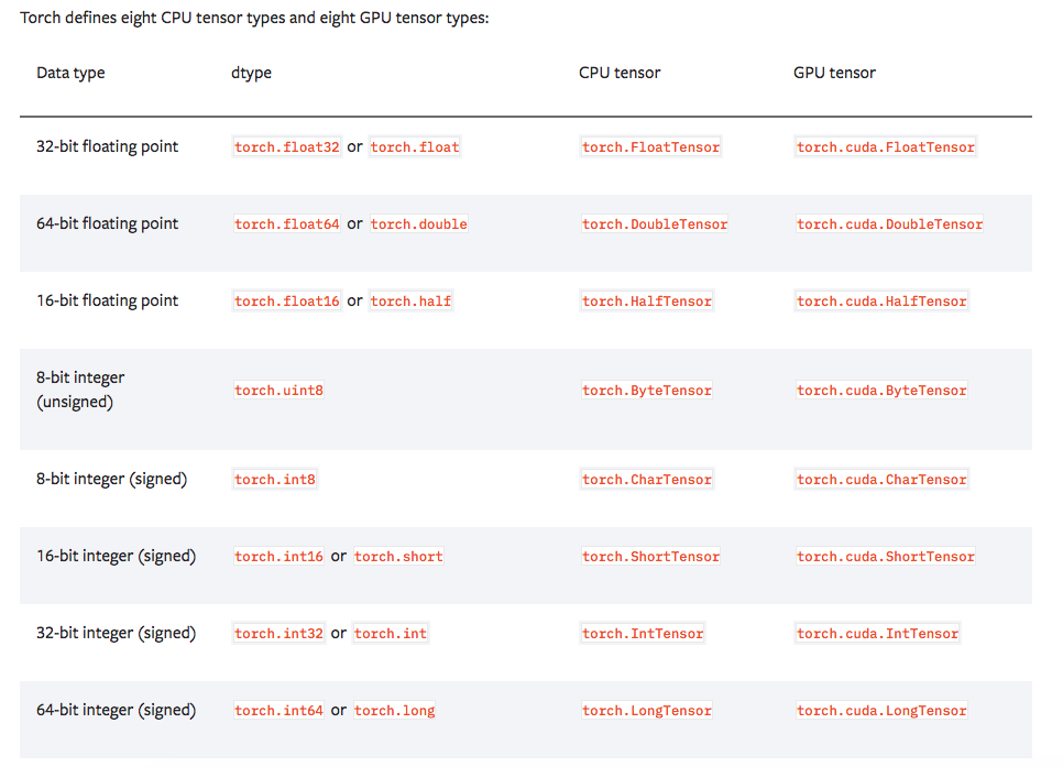
model = model.to(device=device)  # move the model parameters to CPU/GPU

Weight Initialization

def random_weight(shape):
    """
    Create random Tensors for weights; setting requires_grad=True means that we
    want to compute gradients for these Tensors during the backward pass.
    We use Kaiming normalization: sqrt(2 / fan_in)
    """
    if len(shape) == 2:  # FC weight
        fan_in = shape[0]
    else:
        fan_in = np.prod(shape[1:]) # conv weight [out_channel, in_channel, kH, kW]
    # randn is standard normal distribution generator. 
    w = torch.randn(shape, device=device, dtype=dtype) * np.sqrt(2. / fan_in)
    w.requires_grad = True
    return w
# nn.init.kaiming_normal_(self.fc.weight)
----------------------------------------------------------

def zero_weight(shape):
    return torch.zeros(shape, device=device, dtype=dtype, requires_grad=True)
# nn.init.constant_(self.conv1.bias, 0)

The basics

In this section, we’ll go through the basic ideas of PyTorch starting at tensors and computational graphs and finishing at the Variable class and the PyTorch autograd functionality.

Computational graphs

link

The first thing to understand about any deep learning library is the idea of a computational graph. A computational graph is a set of calculations, which are called nodes, and these nodes are connected in a directional ordering of computation. In other words, some nodes are dependent on other nodes for their input, and these nodes in turn output the results of their calculations to other nodes. A simple example of a computational graph for the calculation $a=(b+c)*(c+2)$ can be seen below – we can break this calculation up into the following steps/nodes:

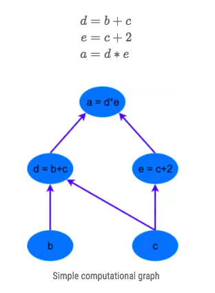
The benefits of using a computational graph is that each node is like its own independently functioning piece of code (once it receives all its required inputs). This allows various performance optimizations to be performed in running the calculations such as threading and multiple processing / parallelism. All the major deep learning frameworks (TensorFlow, Theano, PyTorch etc.) involve constructing such computational graphs, through which neural network operations can be built and through which gradients can be back-propagated.

Tensors

Tensors are matrix-like data structures which are essential components in deep learning libraries and efficient computation. Graphical Processing Units (GPUs) are especially effective at calculating operations between tensors, and this has spurred the surge in deep learning capability in recent times. In PyTorch, tensors can be declared simply in a number of ways:

import torch
x = torch.Tensor(2,3)

This code creates a tensor of size (2, 3) – i.e. 2 rows and 3 columns, filled with zero float values.

We can also create tensors filled random float values:

x = torch.rand(2, 3)

Multiplying tensors, adding them and so forth is straight-forward:

x = torch.ones(2,3)
y = torch.ones(2,3) * 2
print(x + y)
# 3 3 3
# 3 3 3

Another great thing is the numpy slice functionality that is available – for instance y[:, 1]

y[:,1] = y[:,1] + 1
# 2 3 2
# 2 3 2

Numpy Bridge

Converting a Torch Tensor to a NumPy array and vice versa is a breeze. The Torch Tensor and NumPy array will share their underlying memory locations (if the Torch Tensor is on CPU), and changing one will change the other.

Converting a Torch Tensor to a NumPy Array

a = torch.ones(5)
print(a) #tensor([1., 1., 1., 1., 1.])
b = a.numpy()
print(b) #[1. 1. 1. 1. 1.]
a.add_(1)
print(a) #tensor([2., 2., 2., 2., 2.])
print(b) #[2. 2. 2. 2. 2.]

Converting NumPy Array to Torch Tensor

import numpy as np
a = np.ones(5)
b = torch.from_numpy(a)
np.add(a, 1, out=a)
print(a) #[2. 2. 2. 2. 2.]
print(b) #tensor([2., 2., 2., 2., 2.], dtype=torch.float64)

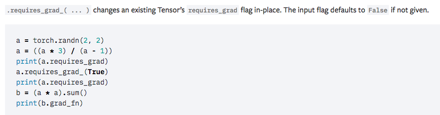
torch.Tensor is the central class of the package. If you set its attribute .requires_grad as True, it starts to track all operations on it. When you finish your computation you can call .backward() and have all the gradients computed automatically. The gradient for this tensor will be accumulated into .grad attribute.

Autograd in Pytorch

link

n any deep learning library, there needs to be a mechanism where error gradients are calculated and back-propagated through the computational graph. This mechanism, called autograd in PyTorch. Pytorch allows automatic gradient computation on the tensor when the .backward() function is called.

import torch
x = torch.ones(2, 2, requires_grad=True)
print(x) 
# tensor([[1., 1.],
#         [1., 1.]],requires_grad=True)

do a tensor operation:

y = x+2
print(y)
#tensor([[3., 3.],
#        [3., 3.]], grad_fn=<AddBackward0>)

y was created as a result of an operation, so it has a grad_fn.

print(y.grad_fn) 
# <AddBackward0 object at 0x7f27857f7c88>

do more operations on y:

z = y * y * 3
out = z.mean()
print(z, out)
#tensor([[27., 27.],
#       [27., 27.]], grad_fn=<MulBackward0>) tensor(27., grad_fn=<MeanBackward0>)

Gradients

Let’s backprop now. Because out contains a single scalar, out.backward() is equivalent to out.backward(torch.tensor(1.)).

out.backward()

Print gradients d(out)/dx

print(x.grad)
#tensor([[4.5000, 4.5000],
#        [4.5000, 4.5000]])

Torch

Tensor

The torch package contains data structures for multi-dimensional tensors and mathematical operations over these are defined.

Creation Ops

tensor

torch.tensor(data, dtype=None, device=None, requires_grad=False, pin_memory=False) → Tensor

Constructs a tensor with data.

topk

topk(k, dim=None, largest=True, sorted=True) -> (Tensor, LongTensor)

Returns the k largest elements of the given input tensor along a given dimension.

If dim is not given, the last dimension of the input is chosen.

If largest is False then the k smallest elements are returned.

A namedtuple of (values, indices) is returned, where the indices are the indices of the elements in the original input tensor.

view

view(*shape) → Tensor

Returns a new tensor with the same data as the self tensor but of a different shape.

size

size() → torch.Size

Returns the size of the self tensor. The returned value is a subclass of tuple.

div

div_(value) → Tensor

Divides each element of the input input with the scalar value and returns a new resulting tensor.

mm

mm(mat2) → Tensor

matrxi multiply. see torch.mm().

torch.from_numpy

torch.from_numpy(ndarray) → Tensor

Creates a Tensor from a numpy.ndarray.

The returned tensor and ndarray share the same memory. Modifications to the tensor will be reflected in the ndarray and vice versa. The returned tensor is not resizable.

Autograd

torch.autograd provides classes and functions implementing automatic differentiation of arbitrary scalar valued functions.

Variable (deprecated)

The Variable API has been deprecated: Variables are no longer necessary to use autograd with tensors. Autograd automatically supports Tensors with requires_grad set to True. Below please find a quick guide on what has changed:

• Variable(tensor) and Variable(tensor, requires_grad) still work as expected, but they return Tensors instead of Variables.
• var.data is the same thing as tensor.data.
• Methods such as var.backward(), var.detach(), var.register_hook() now work on tensors with the same method names.

max

1. torch.max(input) -> Tensor

   Returns the maximum value of all elements in the input tensor.

   >>> a = torch.randn(1, 3)
   >>> a
   tensor([[ 0.6763,  0.7445, -2.2369]])
   >>> torch.max(a)
   tensor(0.7445)

2. torch.max(input, dim, keepdim=False, out=None) -> (Tensor, LongTensor)

   Returns a namedtuple (values, indices) where values is the maximum value of each row of the input tensor in the given dimension dim. And indices is the index location of each maximum value found (argmax).

   If keepdim is True, the output tensors are of the same size as input except in the dimension dim where they are of size 1. Otherwise, dim is squeezed (see torch.squeeze()), resulting in the output tensors having 1 fewer dimension than input.

   • input (Tensor) – the input tensor
   • dim (int) – the dimension to reduce
   • keepdim (bool, optional) – whether the output tensors have dim retained or not. Default: False.
   • out (tuple, optional) – the result tuple of two output tensors (max, max_indices)

   >>> a = torch.randn(4, 4)
   >>> a
   tensor([[-1.2360, -0.2942, -0.1222,  0.8475],
           [ 1.1949, -1.1127, -2.2379, -0.6702],
           [ 1.5717, -0.9207,  0.1297, -1.8768],
           [-0.6172,  1.0036, -0.6060, -0.2432]])
   >>> torch.max(a, 1)
   torch.return_types.max(values=tensor([0.8475, 1.1949, 1.5717, 1.0036]), indices=tensor([3, 0, 0, 1]))

3. torch.max(input, other, out=None) → Tensor

   Each element of the tensor input is compared with the corresponding element of the tensor other and an element-wise maximum is taken.

   >>> a = torch.randn(4)
   >>> a
   tensor([ 0.2942, -0.7416,  0.2653, -0.1584])
   >>> b = torch.randn(4)
   >>> b
   tensor([ 0.8722, -1.7421, -0.4141, -0.5055])
   >>> torch.max(a, b)
   tensor([ 0.8722, -0.7416,  0.2653, -0.1584])

cat

torch.cat(tensors, dim=0, out=None) → Tensor

multinomial

torch.multinomial(input, num_samples, replacement=False, out=None) → LongTensor

understanding

nn

functional

Linear layers

Linear

torch.nn.Linear(in_features, out_features, bias=True)

Applies a linear transformation to the incoming data: $y=x A^{T}+b$.

• in_features – size of each input sample
• out_features – size of each output sample
• bias – If set to False, the layer will not learn an additive bias. Default: True

Variables - Linear.weight and Linear.bias

Convolution layers

Conv2d

torch.nn.Conv2d(in_channels, out_channels, kernel_size, stride=1, padding=0, dilation=1, groups=1, bias=True, padding_mode='zeros')

• dilation controls the spacing between the kernel points; also known as the à trous algorithm. It is harder to describe, but this link has a nice visualization of what dilation does.

Variables - Conv2d.weight and Conv2d.bias

Non-linear activations

Relu

torch.nn.ReLU(inplace=False)

Softmax

torch.nn.Softmax(dim=None)

$$\operatorname{Softmax}\left(x_{i}\right)=\frac{\exp \left(x_{i}\right)}{\sum_{j} \exp \left(x_{j}\right)}\$$

LogSoftmax

torch.nn.LogSoftmax(dim=None)

Applies the Log(Softmax(x)) function to an n-dimensional input Tensor.

CrossEntropyLoss

torch.nn.CrossEntropyLoss(weight=None, size_average=None, ignore_index=-100, reduce=None, reduction='mean')

This criterion combines nn.LogSoftmax() and nn.NLLLoss() in one single class.

Therefore, in network architecture, we should not define a softmax layer.

NLLLoss()

go with LogSoftmax.

Layers

Embedding

torch.nn.Embedding(num_embeddings, embedding_dim, padding_idx=None, max_norm=None, norm_type=2.0, scale_grad_by_freq=False, sparse=False, _weight=None)

Shape

• Input: (*)(∗), LongTensor of arbitrary shape containing the indices to extract
• Output: (, H)(∗,H), where is the input shape and $H=\text{embedding_dim}$

Parameters

• num_embeddings(int) -
• embedding_dim(int) - size of each embedding vector
• padding_idx(int,optional) - If given, pads the output with the embedding vector at padding_idx(initialized to zeros) whenever it encounters the index. understanding

understanding

GRU

torch.nn.GRU(*args, **kwargs)

Parameters

• input_size - The number of expected features in the input x
• hidden_szie - The number of features in the hidden state h
• num_layers - Number of recurrent layers. E.g., setting num_layers=2 would mean stacking two GRUs together to form a stacked GRU, with the second GRU taking in outputs of the first GRU and computing the final results. Default: 1

optim

Adam

torch.optim.Adam(params, lr=0.001, betas=(0.9, 0.999), eps=1e-08, weight_decay=0, amsgrad=False)

[Utils]

DATA

torch.utils.data.DataLoader

torch.utils.data.DataLoader(dataset, batch_size=1, shuffle=False, sampler=None, batch_sampler=None, num_workers=0, collate_fn=<function default_collate>, pin_memory=False, drop_last=False, timeout=0, worker_init_fn=None)

• dataset (Dataset) – dataset from which to load the data.
• batch_size (int, optional) – how many samples per batch to load (default: 1).
• shuffle (bool, optional) – set to True to have the data reshuffled at every epoch (default: False).
• sampler (Sampler, optional) – defines the strategy to draw samples from the dataset. If specified, shufflemust be False.
• batch_sampler (Sampler, optional) – like sampler, but returns a batch of indices at a time. Mutually exclusive with batch_size, shuffle, sampler, and drop_last.
• num_workers (int, optional) – how many subprocesses to use for data loading. 0 means that the data will be loaded in the main process. (default: 0)

torch.utils.data.Sampler

torch.utils.data.Sampler(data_source)

Base class for all Samplers.

Every Sampler subclass has to provide an iter method, providing a way to iterate over indices of dataset elements, and a len method that returns the length of the returned iterators.

torch.utils.data.SubsetRandomSampler

torch.utils.data.SubsetRandomSampler(indices)

Samples elements randomly from a given list of indices, without replacement.

• indices (sequence) – a sequence of indices

Torchvision

Models

import torchvision.models as models
resnet18 = models.resnet18(pretrained=True)
alexnet = models.alexnet(pretrained=True)
squeezenet = models.squeezenet1_0(pretrained=True)
vgg16 = models.vgg16(pretrained=True)
densenet = models.densenet161(pretrained=True)
inception = models.inception_v3(pretrained=True)
googlenet = models.googlenet(pretrained=True)
shufflenet = models.shufflenetv2(pretrained=True)

All pre-trained models expect input images normalized in the same way, i.e. mini-batches of 3-channel RGB images of shape (3 x H x W), where H and W are expected to be at least 224. The images have to be loaded in to a range of [0, 1] and then normalized using mean = [0.485, 0.456, 0.406] and std = [0.229, 0.224, 0.225]. You can use the following transform to normalize:

normalize = transforms.Normalize(mean=[0.485, 0.456, 0.406],
                                 std=[0.229, 0.224, 0.225])

Stop-undating

# Download and load the pretrained SqueezeNet model.
model = torchvision.models.squeezenet1_1(pretrained=True)

# We don't want to train the model, so tell PyTorch not to compute gradients
# with respect to model parameters.
for param in model.parameters():
    param.requires_grad = False

Datasets

All datasets are subclasses of torch.utils.data.Dataset i.e, they have __getitem__ and __len__ methods implemented. Hence, they can all be passed to a torch.utils.data.DataLoader which can load multiple samples parallelly using torch.multiprocessing workers.

imagenet_data = torchvision.datasets.ImageNet('path/to/imagenet_root/')
data_loader = torch.utils.data.DataLoader(imagenet_data,
                                          batch_size=4,
                                          shuffle=True,
                                          num_workers=args.nThreads)

The following datasets are available: MNIST, COCO (Captions and Detection), LSUN, ImageNet, CIFAR etc.

All the datasets have almost similar API. They all have two common arguments: transform and target_transform to transform the input and target respectively.

MNIST

torchvision.datasets.MNIST(root, train=True, transform=None, target_transform=None, download=False)

• root (string) – Root directory of dataset where MNIST/processed/training.pt andMNIST/processed/test.pt exist.
• train (bool, optional) – If True, creates dataset from training.pt, otherwise from test.pt.
• download (bool, optional) – If true, downloads the dataset from the internet and puts it in root directory. If dataset is already downloaded, it is not downloaded again.
• transform (callable, optional) – A function/transform that takes in an PIL image and returns a transformed version. E.g, transforms.RandomCrop
• target_transform (callable, optional) – A function/transform that takes in the target and transforms it.

Transforms

Compose

torchvision.transforms.Compose(transforms)

Composes several transforms together.

• transforms (list of Transform objects) – list of transforms to compose.

transforms.Compose([
   transforms.CenterCrop(10),
   transforms.ToTensor(),
])

Resize

torchvision.transforms.Resize(size, interpolation=2)

Resize the input PIL Image to the given size.

• size (sequence or int) – Desired output size. If size is a sequence like (h, w), output size will be matched to this. If size is an int, smaller edge of the image will be matched to this number. i.e, if height > width, then image will be rescaled to (size * height / width, size)
• interpolation (int, optional) – Desired interpolation. Default is PIL.Image.BILINEAR

torchvision.transforms.``Scale(args*, *kwargs*) is deprecated in favor of Resize.

ToTensor

torchvision.transforms.ToTensor()

Convert a PIL Image or numpy.ndarray to tensor.

Normalize

torchvision.transforms.Normalize(mean, std, inplace=False)

Normalize a tensor image with mean and standard deviation. Given mean: (M1,...,Mn) and std: (S1,..,Sn) for nchannels, this transform will normalize each channel of the input torch.*Tensor i.e. input[channel] =(input[channel] - mean[channel]) / std[channel]

This transform acts out of place, i.e., it does not mutates the input tensor.

Lambda

torchvision.transforms.Lambda(lambd)

Apply a user-defined lambda as a transform.

• lambd (function) – Lambda/function to be used for transform.

HyperParameters Search

source

Visualization

source

Pytorch in Practice

Char_Level Names Classification

import string,unicodedata
import glob
from collections import defaultdict
import torch
import torch.nn as nn
import torch.nn.functional as F
import torch.optim as optim
import numpy as np

all_letters = string.ascii_letters + " .,;'"
n_letters = len(all_letters)
print(n_letters, all_letters)

# Turn a Unicode string to plain ASCII, thanks to http://stackoverflow.com/a/518232/2809427
def unicode_to_ascii(s):
    return ''.join(
        c for c in unicodedata.normalize('NFD', s)
        if unicodedata.category(c) != 'Mn'
        and c in all_letters
    )

print(unicode_to_ascii('Ślusàrski'))
print(os.getcwd())

all_files = glob.glob('/content/colabdataset/ColabDataset/names/*.txt')
print(all_files)
Country2Name = defaultdict(list)
Countries = []
for file in all_files:
  country = file.split('/')[-1][:-4]
  Countries.append(country)
  print(country)
  f = open(file)
  lines = f.readlines()
  names = []
  for line in lines:
    names.append(unicode_to_ascii(line.replace('\n','')))
  Country2Name[country] = names
print(Country2Name['Chinese'][:10])

def str2tensor(name):
  time_step = len(name)
  feature_dim = n_letters
  batch_size = 1
  tensor = torch.zeros(time_step,batch_size,feature_dim)
  for idx,val in enumerate(name):
    tensor[idx,0,all_letters.index(val)] = 1
  tensor = tensor.permute(1,0,2)
  return tensor

def get_training_pair():
  country_label = np.random.choice(Countries)
  names = np.random.choice(Country2Name[country_label])
  tensor_names = str2tensor(names)
  tensor_label = torch.tensor([Countries.index(country_label)])
  return tensor_names,tensor_label

class rnn_classifier(nn.Module):
  def __init__(self,input_size,hidden_size,output_size):
    super(rnn_classifier,self).__init__()
    self.input_size = input_size
    self.hidden_size = hidden_size
    self.output_size = output_size
    
    self.embed = nn.Embedding(input_size,hidden_size)
    # input of shape (seq_len, batch, input_size)
    # output of shape (seq_len, batch, num_directions * hidden_size)
    self.lstm = nn.LSTM(self.input_size,self.hidden_size,batch_first=True) 
    self.fc = nn.Linear(self.hidden_size,self.output_size)
  
  def forward(self,input):
    hidden,(_,_) = self.lstm(input) #AttributeError: 'tuple' object has no attribute 'dim' if hidden = self.lstm(input) 
    output = self.fc(hidden)
    return output

n_hidden = 128
rnn = rnn_classifier(n_letters,n_hidden,len(Countries))
criterion = nn.CrossEntropyLoss()
opt = torch.optim.SGD(rnn.parameters(),lr=0.005)

def train(input,output):
  opt.zero_grad()
  pred = rnn(input)
  pred = pred[:,-1,:].squeeze(dim=1)
  loss = criterion(pred,output)
  loss.backward()
  opt.step()
  return pred,loss.item()

n_epochs = 100000
print_every = 5000
current_loss = 0
for epoch in range(n_epochs):
  input,output = get_training_pair()
  pred,loss = train(input,output)
  current_loss += loss
  if epoch % print_every == 0:
    print(epoch,'/',n_epochs,loss)
    
def get_testing_pair():
  country_label = np.random.choice(Countries)
  names = np.random.choice(Country2Name[country_label])
  tensor_names = str2tensor(names)
  tensor_label = torch.tensor([Countries.index(country_label)])
  return names,country_label,tensor_names,tensor_label

def prediction(name_tensor,names,gt):
  pred = rnn(name_tensor)
  pred = pred[:,-1,:].squeeze(1)
  _,idx = torch.max(pred.data,1)
  return Countries[idx]

n = 100
c = 0
for t in range(100):
  names,country_label,tensor_names,tensor_label = get_testing_pair() 
  pred = prediction(tensor_names,names,country_label)
  print('name is {}, the prediction is {}, while the gound_t is {}'.format(names,pred,country_label))
  if pred==country_label:
    c += 1
print("Acurracy is {}".format(c/n))

There are several points needed the attention:

1. Input data and groundtruth

   The input data should be in the size (time_steps, batch_size, feature_dim) for the original LSTM function. But if you specify the parameter batch_first in LSTM, then you need to switch the dimentaion to (batch_size, time_steps, feature_dim).

   As for the groundtruth, it should be a scalar instead of a one-hot label if we are dealing with the classification problem, whose size should be (batch_size,1). For example, if the batch_size is 1, so one possilbility could be [1] instead of 1.

   In this case, we usually use CrossEntropyLoss or NLLLoss.

2. Loss function

   If in the model definition we have a layer called LogSoftmax, then we should use CrossEntropyLoss.

3. Training function

   For LSTM, the input of shape should be [seq_len, batch, input_size], while the output shape would be [seq_len, batch, hidden_size]. And then going through a Linear layer, the output size should be [seq_len, batch, output_size]. Here the output_size is class number. But we only need the last element of output, which means output[-1,:,:]. This is because for each time step, there is always a output.

4. Prediction

   When testing, we should reshape the prediction to [batch_size,output_size], then we can use val,idx = torch.max(prediction,1) for printing.

5. xxx

6. ​

Reference

Deep Learning With PyTorch

A PyTorch tutorial – deep learning in Python

jcjohnson’s PyTorch examples