NLP-Word2Vec

Word embedding, i.e., vector representations of a particular word and also called word vectoring, is important in NLP. It is capable of capturing context of a word in a document, semantic and syntactic similarity, relation with other words, etc.

Word2Vec, as one of the most popular technique to learn word embeddings using shallow neural network, includes:

• 2 algorithms: continuous bag-of-words (CBOW) and skip-gram. CBOW aims to predict a center word from the surrounding context in terms of word vectors. Skip-gram does the opposite, and predicts the distribution (probability) of context words from a center word.
• 2 training methods: negative sampling and hierarchical softmax. Negative sampling defines an objective by sampling negative examples, while hierarchical softmax defines an objective using an efficient tree structure to compute probabilities for all the vocabulary.

Why do we need them?

Consider the following similar sentences: Have a good day and Have a great day. They hardly have different meaning. If we construct an exhaustive vocabulary (let’s call it V), it would have V = {Have, a, good, great, day}.

Now, let us create a one-hot encoded vector for each of these words in V. Length of our one-hot encoded vector would be equal to the size of V (=5). We would have a vector of zeros except for the element at the index representing the corresponding word in the vocabulary. That particular element would be one. The encodings below would explain this better.

Have = [1,0,0,0,0]; a=[0,1,0,0,0] ; good=[0,0,1,0,0]; great=[0,0,0,1,0] ; day=[0,0,0,0,1]( represents transpose)

If we try to visualize these encodings, we can think of a 5 dimensional space, where each word occupies one of the dimensions and has nothing to do with the rest (no projection along the other dimensions). This means ‘good’ and ‘great’ are as different as ‘day’ and ‘have’, which is not true.

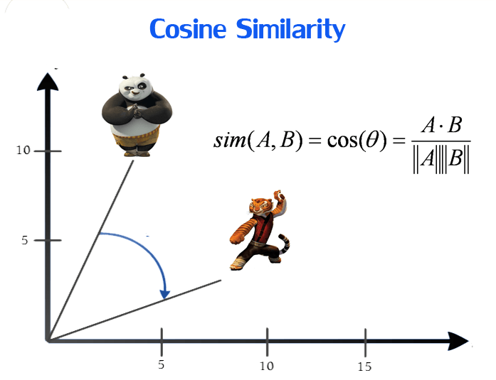
Our objective is to have words with similar context occupy close spatial positions. Mathematically, the cosine of the angle between such vectors should be close to 1, i.e. angle close to 0.

Here comes the idea of generating distributed representations. Intuitively, we introduce some dependence of one word on the other words. The words in context of this word would get a greater share of this dependence. In one hot encoding representations, all the words are independent of each other, as mentioned earlier.

How does Word2Vec work?

Word2Vec is a method to construct such an embedding. It can be obtained using two methods (both involving Neural Networks): Skip Gram and Common Bag Of Words (CBOW)

CBOW Model

This method takes the context of each word as the input and tries to predict the word corresponding to the context.

Let the input to the Neural Network be the word, great. Notice that here we are trying to predict a target word (day) using a single context input word great. More specifically, we use the one hot encoding of the input word and measure the output error compared to one hot encoding of the target word (day). In the process of predicting the target word, we learn the vector representation of the target word.

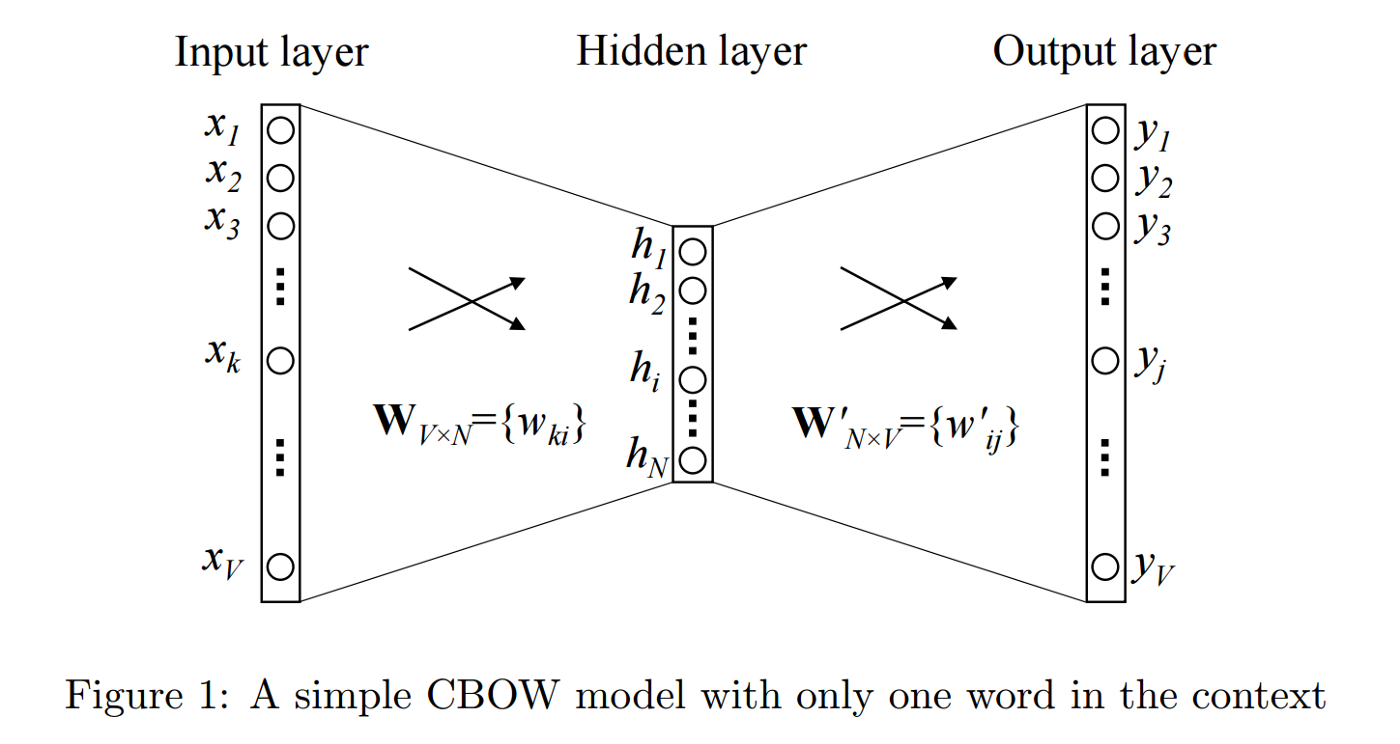
Note: input is the one-hot vector of one word.

The input or the context word is a one hot encoded vector of size V. The hidden layer contains N neurons and the output is again a V length vector with the elements being the softmax values.

The hidden layer neurons just copy the weighted sum of inputs to the next layer. There is no activation like sigmoid, tanh or ReLU. The only non-linearity is the softmax calculations in the output layer.

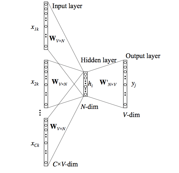
But, the above model used a single context word to predict the target. We can use multiple context words to do the same.

Skip-Gram Model

We can use the target word (whose representation we want to generate) to predict the context and in the process, we produce the representations.

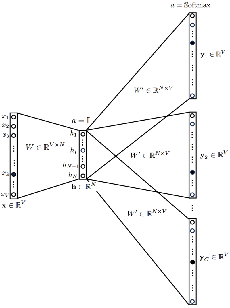
We input the target word into the network. The model outputs C probability distributions. What does this mean? For each context position, we get C probability distributions of V probabilities, one for each word.

The Hidden Layer

For our example, we’re going to say that we’re learning word vectors with 300 features. So the hidden layer is going to be represented by a weight matrix with 10,000 rows (one for every word in our vocabulary) and 300 columns (one for every hidden neuron).

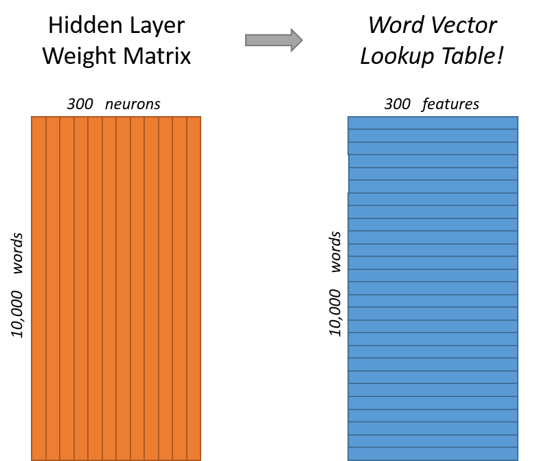
So the end goal of all of this is really just to learn this hidden layer weight matrix – the output layer we’ll just toss when we’re done!

Now, you might be asking yourself–“That one-hot vector is almost all zeros… what’s the effect of that?” If you multiply a 1 x 10,000 one-hot vector by a 10,000 x 300 matrix, it will effectively just select the matrix row corresponding to the “1”. Here’s a small example to give you a visual.

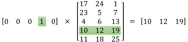
This means that the hidden layer is operating as a lookup table. The output of the hidden layer is just the “word vector” for the input word.

Intuition

Ok, are you ready for an exciting bit of insight into this network?

If two different words have very similar “contexts” (that is, what words are likely to appear around them), then our model needs to output very similar results for these two words. And one way for the network to output similar context predictions for these two words is if the word vectors are similar. So, if two words have similar contexts, then our network is motivated to learn similar word vectors for these two words! Ta da!

say we have two words, their word embedding are A and B. The hidden-output weight matrix is HO, so the outputs are A*HO and B*HO. Because these two words have similar contexts, so the groundtruth target should be same. which result in A*HO = B*HO, meaning A and B have to be similar.

And what does it mean for two words to have similar contexts? I think you could expect that synonyms like “intelligent” and “smart” would have very similar contexts. Or that words that are related, like “engine” and “transmission”, would probably have similar contexts as well.

This can also handle stemming for you – the network will likely learn similar word vectors for the words “ant” and “ants” because these should have similar contexts.

Loss Function

Say we have a word documents with $T$ words, our task is to predict context words within a window of fixed size $m$, given center word $w_j$:

$$max \ L(\theta)=max \ \prod_{t=1}^{T} \prod_{-m \leq j \leq m \atop j \neq 0} P\left(w_{t+j} | w_{t} ; \theta\right)$$

to simplify it:

$$min \ J(\theta)=min \ -\frac{1}{T} \log L(\theta)=min \ -\frac{1}{T} \sum_{t=1}^{T} \sum_{-m \leq j \leq m \atop j \neq 0} \log P\left(w_{t+j} | w_{t} ; \theta\right)$$

Here, we transform max to min by put a negative sign in front of the formula.

In order to calculate $P\left(w_{t+j} | w_{t} ; \theta\right)$, we need to introduce two vectors for each word in the document:

• $v_w$ when $w$ is a center word
• $u_w$ when $w$ is a context word

Then for a center word $c$ and a context word $o$:

$$P(o | c)=\frac{\exp \left(u_{o}^{T} v_{c}\right)}{\sum_{w \in V} \exp \left(u_{w}^{T} v_{c}\right)}$$

which equals the softmax function if we take $x_i=u_{o}^{T} v_{c}$,

$$\operatorname{softmax}\left(x_{i}\right)=\frac{\exp \left(x_{i}\right)}{\sum_{j=1}^{n} \exp \left(x_{j}\right)}=p_{i}$$

The softmax function maps arbitrary values $x_i$ to a probability distribution $p_i$,

• “max” because amplifies probability of largest $x_i$,
• “soft” because still assigns some probability to smaller $x_i$

Gradient

Say we want to calculate the derivative of center vector $v_c$,

$$\\ \begin{equation} \begin{aligned} \frac{\partial}{\partial v_c}logP(o | c)&= \frac{\partial}{\partial v_c}log \frac{\exp \left(u_{o}^{T} v_{c}\right)}{\sum_{w \in V} \exp \left(u_{w}^{T} v_{c}\right)} \\ &=\frac{\partial}{\partial v_c}log{\exp \left(u_{o}^{T} v_{c}\right)}-\frac{\partial}{\partial v_c}log {\sum_{w \in V} \exp \left(u_{w}^{T} v_{c}\right)} \\ &=\frac{\partial}{\partial v_c}{ \left(u_{o}^{T} v_{c}\right)} - \frac{1}{\sum_{w \in V}\exp(u_{w}^{T}v_{c})}\frac{\partial}{\partial v_c}{\sum_{x \in V} \exp \left(u_{x}^{T} v_{c}\right)} \\ &= u_o - \frac{1}{\sum_{w \in V} \exp \left(u_{w}^{T} v_{c}\right)}{\sum_{x \in V}}\frac{\partial}{\partial v_c}\exp \left(u_{x}^{T} v_{c}\right) \\ &=u_o - \frac{1}{\sum_{w \in V} \exp \left(u_{w}^{T} v_{c}\right)}{\sum_{x \in V}}\exp \left(u_{x}^{T} v_{c}\right)\frac{\partial}{\partial v_c}(u_x^Tv_c) \\ &=u_o - \frac{1}{\sum_{w \in V} \exp \left(u_{w}^{T} v_{c}\right)}{\sum_{x \in V}}\exp \left(u_{x}^{T} v_{c}\right)(u_x) \\ &=u_o-\sum_{w\in V}P(o|c)u_w \end{aligned} \end{equation}$$

Here $\sum_{w\in V}P(o|center)u_w$ is the expected context word by our trained model, and $u_o$ is our target context, it is like the difference between the target and prediction.

We can treat $u_0$ as we choose the target row from contect matrix $U$, which is $U^T\cdot y$; as for $u_w$, we can see it as we also choose a row from context matrix, but which row? Actually, it is each row of the matrix and average them. Because $P(o|c)$ is the prediction, which is the output of our model, so we can treat it as $\hat y$. Therefor $\sum_{w\in V}P(o|c)u_w=U^T \cdot \hat y$ , so the gradient for center word vector is:

$$\frac{\partial}{\partial v_c}logP(o | c)= U^T \cdot (\hat y-y)$$

where $U$ is one of the learned weights.

Then we need to calculate the derivative for context vector $u_w$:

if $w=o$, then:

$$\begin{array}{c}{\frac{\partial logP(o | c)}{\partial \boldsymbol{u}_{w}}} \\ {=-\boldsymbol{v}_{c}+\frac{1}{\sum_{w=1}^{V} \exp \left(\boldsymbol{u}_{w}^{T} \boldsymbol{v}_{c}\right)} \frac{\partial \sum_{w=1}^{V} \exp \left(\boldsymbol{u}_{w}^{T} \boldsymbol{v}_{c}\right)}{\partial \boldsymbol{u}_{o}}} \\ {=-\boldsymbol{v}_{c}+\frac{1}{\sum_{w=1}^{V} \exp \left(\boldsymbol{u}_{w}^{T} \boldsymbol{v}_{c}\right)} \frac{\partial \exp \left(\boldsymbol{u}_{o}^{T} \boldsymbol{v}_{c}\right)}{\partial \boldsymbol{u}_{o}}} \\ {=-\boldsymbol{v}_{c}+\frac{\exp \left(\boldsymbol{u}_{o}^{T} \boldsymbol{v}_{c}\right)}{\sum_{w=1}^{V} \exp \left(\boldsymbol{u}_{w}^{T} \boldsymbol{v}_{c}\right)} \boldsymbol{v}_{c}} \\ {=(P(O=o | C=c)-1) \boldsymbol{v}_{c}}\end{array}$$

if $w \ne o$,

$$\begin{array}{c}{\frac{\partial logP(o | c)}{\partial \boldsymbol{u}_{w}}}\\ {=\frac{\exp \left(\boldsymbol{u}_{w}^{T} \boldsymbol{v}_{c}\right)}{\sum_{w=1}^{V} \exp \left(\boldsymbol{u}_{w}^{T} \boldsymbol{v}_{c}\right)} \boldsymbol{v}_{c}} \\ {=P(O=w | C=c) \boldsymbol{v}_{c}}\end{array}$$

Similarly, we can combine $P(O=o | C=c)-1$ and $P(O=o | C=c)$ as $\hat y - y$,

$$\frac{\partial \log p(o | c)}{\partial u_{o}}=(\hat y-y) \cdot v_{c}$$

Negative sampling

You may have noticed that the skip-gram neural network contains a huge number of weights… For our example with 300 features and a vocab of 10,000 words, that’s 3M weights in the hidden layer and output layer each! Training this on a large dataset would be prohibitive.

The main idea of negative sampling is to train binary logistic regressions for a true pair (center word and word in its context window) versus several noise pairs (the center word paired with a random word)

Negative sampling addresses this by having each training sample only modify a small percentage of the weights, rather than all of them. Here’s how it works.

Assume that $K$ negative samples (words) are drawn from the vocabulary. For simplicity of notation we shall refer to them as $w_1,w_2,..,w_k$ and their outside vectors as $u_1,u_2,…,u_k$. Note that $o \notin \{w_1,w_2,…,w_k\}$. For a center word $c$ and an outside word $o$, the negative sampling loss function is given by:

$$J_{\mathrm{neg}-\text { sample }}\left(\boldsymbol{v}_{c}, o, \boldsymbol{U}\right)=-\log \left(\sigma\left(\boldsymbol{u}_{o}^{\top} \boldsymbol{v}_{c}\right)\right)-\sum_{k=1}^{K} \log \left(\sigma\left(-\boldsymbol{u}_{k}^{\top} \boldsymbol{v}_{c}\right)\right)$$

for a sample $w_1,…,w_k$, where $\sigma(\cdot)$ is the sigmoid function. The idea is to maximize probability that real outside word appears, minimize prob. that random words appear around center word.

Gradient

For center word vector $v_c$:

$$\begin{array}{c}{\frac{\partial J_{\text {neg-sample}}\left(\boldsymbol{v}_{c}, o, \boldsymbol{U}\right)}{\partial \boldsymbol{v}_{c}} \log \left(\sigma\left(-\boldsymbol{u}_{k}^{T} \boldsymbol{v}_{c}\right)\right)} \\ {=\frac{\partial\left(-\log \left(\sigma\left(\boldsymbol{u}_{o}^{T} \boldsymbol{v}_{c}\right)\right)-\sum_{k=1}^{K} \log \left(\sigma\left(-\boldsymbol{u}_{k}^{T} \boldsymbol{v}_{c}\right)\right)\right)}{\partial \boldsymbol{v}_{c}}} \\ {=-\frac{\sigma\left(\boldsymbol{u}_{o}^{T} \boldsymbol{v}_{c}\right)\left(1-\sigma\left(\boldsymbol{u}_{o}^{T} \boldsymbol{v}_{c}\right)\right)}{\sigma\left(\boldsymbol{u}_{o}^{T} \boldsymbol{v}_{c}\right)} \frac{\partial \boldsymbol{u}_{o}^{T} \boldsymbol{v}_{c}}{\partial \boldsymbol{v}_{c}}-\sum_{k=1}^{K} \frac{\partial \log \left(\sigma\left(-\boldsymbol{u}_{k}^{T} \boldsymbol{v}_{c}\right)\right)}{\partial \boldsymbol{v}_{c}}} \\ {=-\left(1-\sigma\left(\boldsymbol{u}_{o}^{T} \boldsymbol{v}_{c}\right)\right) \boldsymbol{u}_{o}+\sum_{k=1}^{K}\left(1-\sigma\left(-\boldsymbol{u}_{k}^{T} \boldsymbol{v}_{c}\right)\right) \boldsymbol{u}_{k}}\end{array}$$

For outside target word vector $u_o$:

$$=\frac{\partial\left(-\log \left(\sigma\left(\boldsymbol{u}_{o}^{T} \boldsymbol{v}_{c}\right)\right)\right.}{\partial \boldsymbol{u}_{o}}=-\left(1-\sigma\left(\boldsymbol{u}_{o}^{T} \boldsymbol{v}_{c}\right)\right) \boldsymbol{v}_{c}$$

For sampling outside word vector $u_w$:

$$=\frac{\partial\left(-\log \left(\sigma\left(-\boldsymbol{u}_{k}^{T} \boldsymbol{v}_{c}\right)\right)\right.}{\partial \boldsymbol{u}_{k}}=\left(1-\sigma\left(-\boldsymbol{u}_{k}^{T} \boldsymbol{v}_{c}\right)\right) \boldsymbol{v}_{c}$$

Numpy Implementation

def skipgram(currentCenterWord, windowSize, outsideWords, word2Ind,
             centerWordVectors, outsideVectors, dataset,
             word2vecLossAndGradient=naiveSoftmaxLossAndGradient):
    '''
    :param currentCenterWord: one current center word
    :param windowSize: integer, context window size
    :param outsideWords: list of no more than 2*windowSize strings, the outside words
    :param word2Ind: a dictionary that maps words to their indices in
              the word vector list
    :param centerWordVectors: center word vectors (as rows) for all words in vocab
    :param outsideVectors: outside word vectors (as rows) for all words in vocab
    :param dataset:
    :param word2vecLossAndGradient: he loss and gradient function for
                               a prediction vector given the outsideWordIdx
                               word vectors, could be one of the two
                               loss functions you implemented above.
    :return:
    loss -- the loss function value for the skip-gram model
    gradCenterVecs -- the gradient with respect to the center word vectors
    gradOutsideVectors -- the gradient with respect to the outside word vectors
    '''
    loss = 0.0
    gradCenterVecs = np.zeros(centerWordVectors.shape)
    gradOutsideVectors = np.zeros(outsideVectors.shape)

    idx = word2Ind[currentCenterWord]
    center_word_vector = centerWordVectors[idx]
    for outside_word in outsideWords:
        outside_word_idx = word2Ind[outside_word]
        loss_, gradCenterVec_, gradOutsideVecs_ = word2vecLossAndGradient(center_word_vector, outside_word_idx,
                                                                          outsideVectors, dataset)

        loss += loss_
        gradCenterVecs[idx] += gradCenterVec_
        gradOutsideVectors += gradOutsideVecs_

    return loss, gradCenterVecs, gradOutsideVectors

def naiveSoftmaxLossAndGradient(centerWordVec,outsideWordIdx,outsideVectors):
    '''
    :param centerWordVec: shape=(D,)
    :param outsideWordIdx: target word index
    :param outsideVectors: shape=(W,D)
    :return:
    '''

    W,D = outsideVectors.shape
    scores = centerWordVec.dot(outsideVectors.T)
    prob = softmax(scores)

    loss = -1*np.log(prob)[outsideWordIdx]

    target = np.zeros(W)
    target[outsideWordIdx] = 1
    gradCenterVec = outsideVectors.T.dot(prob-target)
    gradOutsideVecs = (prob-target).reshape(-1,1).dot(centerWordVec.reshape((1,-1)))

    return loss, gradCenterVec, gradOutsideVecs

def negSamplingLossAndGradient(centerWordVec,outsideWordIdx,outsideVectors,dataset,K=10):
    '''
    :param centerWordVec: size [D,]
    :param outsideWordIdx: size [1,]
    :param outsideVectors: size [W,D]
    :param dataset:
    :param K:
    :return:
    '''
    negSampleWordIndices = getNegativeSamples(outsideWordIdx, dataset, K)

    indices = [outsideWordIdx] + negSampleWordIndices

    gradCenterVec = np.zeros_like(centerWordVec)
    gradOutsideVecs = np.zeros_like(outsideVectors)
    loss = 0

    scores1 = centerWordVec.dot(outsideVectors[outsideWordIdx].T)
    scores2 = np.dot(outsideVectors[outsideWordIdx],centerWordVec)
    prob = sigmoid(scores2)
    loss -= np.log(prob)

    gradCenterVec += (prob-1)*outsideVectors[outsideWordIdx]
    gradOutsideVecs[outsideWordIdx] += (prob-1)* centerWordVec

    for i in range(K):
        idx = indices[i+1]
        s = centerWordVec.dot(-1*outsideVectors[idx].T)
        p = sigmoid(s)
        loss -= np.log(p)

        gradCenterVec += (1-p)*outsideVectors[idx]
        gradOutsideVecs[idx] += (1-p)*centerWordVec

    return loss, gradCenterVec, gradOutsideVecs

Reference

Introduction to Word Embedding and Word2Vec

Word2Vec Tutorial - The Skip-Gram Model

An Intuitive Understanding of Word Embeddings: From Count Vectors to Word2Vec - calculation examples

Stanford CS224d) Deep Learning and NLP课程笔记（二）：word2vec