DP-Clasical CNNs

In this post, we’ll go into summarizing a lot of the new and important developments in the field of computer vision and convolutional neural networks.

The 9 Deep Learning Papers You Need To Know About (Understanding CNNs Part 3)

Alex

AlexNet is introduced in the seminal paper ImageNet Classification with Deep Convolutional Neural Networks, which is a deep convolutional neural network and kicked ass on the ImageNet LSVRC-2010 contest. AlexNet does a pretty good job classifying the 1.2 million high-resolution images into 1000 different classes. Actually, top-1 and top-5 error rate of 37.5% and 17.5% are achieved on the test data, which is way better than the previous state-of-the-art. In this article, I will introduce what AlexNet is, namely the network architecture, how they deal with overfitting, and evaluation results.

Architecture

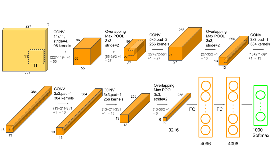
The picture above shows the architecture of AlexNet.We can eyeball the graph and find that AlexNet contains eight layers  —  five convolutional and three fully-connected layers. ref

Input: $227 \times 227 \times 3$ images

1st Convolutional Layers: 96 kernels with kernel size $11 \times 11$, strides=4, pad=0, activation=”relu”

$55 \times 55 \times 96$ feature maps

total number of parameters = $(11113)*96=35K$.

Then $3 \times 3$ Max Pooling (strides=2)

bO PARAMETERS.

$27 \times 27 \times 96$ feature maps

1. Max Pooling layers are usually used to downsample the width and height of the tensors, keeping the depth same.
2. ReLU is chosen because of its non-saturating-nonlinearity peoperty, which is $f(x)=max(x,0)$, resulting in the benefits that deep convolutional neural networks with ReLUs train several times faster than their equivalents with tanh units.
3. Compared with the previous state-of-the-art, the overlapping pooling instead of nonoverlapping pooling is utilized, which helps improve the classification accuray.

2nd Convolutional Layers: 256 kernels with kernel size $5 \times 5$, strides=1, pad=2, activation=”relu”

pad=2 are used to keep output maps having smae size with input maps.

$27 \times 27 \times 256$ feature maps

Then $3 \times 3$ Max Pooling (strides=2)

$13 \times 13 \times 256$ feature maps

3rd Convolutional Layers: 384 kernels with kernel size $3 \times 3$, strides=1, pad=, activation=”relu”1

$13 \times 13 \times 384$ feature maps

4th Convolutional Layers: 384 kernels with kernel size $3 \times 3$, strides=1, pad=1, activation=”relu”

$13 \times 13 \times 384$ feature maps

5th Convolutional Layers: 256 kernels with kernel size $3 \times 3$, strides=1, pad=1, activation=”relu”

$13 \times 13 \times 384$ feature maps

Then $3 \times 3$ Max Pooling (strides=2)

$6 \times 6 \times 256$ feature maps

6th Fully-Connected Layers: 4096 neurons, activation=’tanh’

7th Fully-Connected Layers: 4096 neurons, activation=’tanh’

8th Fully-Connected Layers: 1000 neurons (since there 1000 classes), activation=’softmax’

Implementation

Alright, let’s write a program that learns how to recognize images using cifar10 dataset. We’ll do this with a short keras program.

Let me explain the dataset cifar10 firstly before going to the architecture implementation. Instead of all images, we just use two categories, i.e. cat and dog. Dog vs Cat consists of 12500 training cat images and 12500 training dog images. We are going to use 1000 cat images and 1000 dog images as training dataset while 400 cat images and 400 dog images as testing datasets. Here’s the code we use to organize the training and test datasets.

import os
import cv2

inpath = "/Users/daniel/Documents/all/train/"

outcatTra = "/Users/daniel/Documents/all/Training/cats/"

outdogTra = "/Users/daniel/Documents/all/Training/dogs/"

outcatTest = "/Users/daniel/Documents/all/Testing/cats/"

outdogTest = "/Users/daniel/Documents/all/Testing/dogs/"

os.makedirs(outcatTra,exist_ok=True)
os.makedirs(outdogTra,exist_ok=True)
os.makedirs(outcatTest,exist_ok=True)
os.makedirs(outdogTest,exist_ok=True)

for i in range(1000):
    cat = cv2.imread(inpath+"cat.%d.jpg"%i)
    dog = cv2.imread(inpath+"dog.%d.jpg"%i)

    cv2.imwrite(outcatTra+"cat.%d.jpg"%i,cat)
    cv2.imwrite(outdogTra+"dog.%d.jpg"%i,dog)

for i in range(400):
    j = 4000+i
    cat = cv2.imread(inpath + "cat.%d.jpg" % j)
    dog = cv2.imread(inpath + "dog.%d.jpg" % j)

    cv2.imwrite(outcatTest + "cat.%d.jpg" % i, cat)
    cv2.imwrite(outdogTest + "dog.%d.jpg" % i, dog)

After running the codes, we will have the dataset organization like this:

Data/
    Training/
            cats/
                cat.0.jpg
                cat.1.jpg
                .
                .
                .
                cat.999.jpg
            dogs/
                dog.0.jpg
                dog.1.jpg
                .
                .
                .
                dog.999.jpg
    Testing/
           cats/
               cat.0.jpg
               cat.1.jpg
               .
               .
               .
               cat.399.jpg
           dogs/
               dog.0.jpg
               dog.1.jpg
               .
               .
               .
               dog.399.jpg

Then, I am going to introduce ImageDataGenerator, which is employed to argument dataset.

from keras.preprocessing.image import ImageDataGenerator

# https://blog.csdn.net/jacke121/article/details/79245732
class DataLoader():
    def __init__(self,img_res=(227, 227)):
        self.img_res = img_res

    def load_batch(self,batch_size):
        train_datagen = ImageDataGenerator(
            shear_range= 0.2,
            zoom_range= 0.2,
            horizontal_flip=True
        )
        test_datagen = ImageDataGenerator()
        train_generator = train_datagen.flow_from_directory(
            './dataset_path/',
            batch_size=batch_size,
            shuffle=True,
            target_size=self.img_res,
            class_mode='categorical'
        )
        validation_generator = test_datagen.flow_from_directory(
            './dataset_path/',
            batch_size=batch_size,
            target_size=self.img_res,
            shuffle=True,
            class_mode='categorical'
        )

        return train_generator,validation_generator

img_size is used to resize all the input image so that they have the same width and height. Then we create an ImageDataGenerator instance with specified parameters, where:

• shear_range is used to sheer images and its value is shear angle in counter-clockwise direction in degrees.
• zoom_range is is used for image zoom and a value greater than 1 corresponds to image amplification otherwise image reduction.
• horizontal_flip is used to flip inputs horizontally.

Then we create a data generator by using the instance above. Note that we should explicitly point out the dataset directory, which contain one subdirectory per class. Here we generate train_generator and validation_generator.

Let me explain the core features of the AlexNet code, before giving a full listing. The centerpiece is a AlexNet class, which we use to represent a AlexNet. Here is the code we use to initialize a AlexNet object.

from keras import layers
from keras.models import Model
from keras import backend as K
from keras.optimizers import Adam
from data_load import DataLoader
class AlexNet():
    def __init__(self):
        self.height = 227
        self.width = 227
        self.channels = 3
        self.img_shape = (self.height,self.width,self.channels)
        self.nb_classes = 2
        self.mean_flag = False
        self.data_loader = DataLoader(img_res=(self.height, self.width))
        optimizer = Adam()

        self.alexnet = self.make_model()
        self.alexnet.compile(loss='categorical_crossentropy',
                             optimizer=optimizer,
                             metrics=['accuracy'])

In this code, we make all images share the same height and weight, i.e., 227, and the input images are three channels. Since we only have two categories, so nb_classes=2. Then we create a data loader class. By self.alexnet = self.make_model(), we build a AlexNet and in order to train the network, we use categorical_crossentropy as loss and use Adam to optimize the network. Here is the code for make_model method:

def make_model(self):
        input = layers.Input(shape=self.img_shape)
        if self.mean_flag:
            pass
        x = layers.Conv2D(96,kernel_size=11,strides=4,activation='relu',padding='same')(input)
        x = layers.MaxPooling2D(pool_size=(3,3),strides=2)(x)
        x = layers.BatchNormalization()(x)

        x = layers.Conv2D(256, kernel_size=5, activation='relu',padding='same')(x)
        x = layers.MaxPooling2D(pool_size=(3, 3), strides=2)(x)
        x = layers.BatchNormalization()(x)

        x = layers.Conv2D(384, kernel_size=3, activation='relu',padding='same')(x)
        x = layers.Conv2D(384, kernel_size=3, activation='relu',padding='same')(x)

        x = layers.Conv2D(256, kernel_size=3, activation='relu',padding='same')(x)
        x = layers.MaxPooling2D(pool_size=(3, 3), strides=2)(x)
        x = layers.BatchNormalization()(x)

        x = layers.Flatten()(x)
        x = layers.Dense(4096,activation='tanh')(x)
        x = layers.Dropout(0.5)(x)
        x = layers.Dense(4096,activation='tanh')(x)
        x = layers.Dropout(0.5)(x)
        output = layers.Dense(self.nb_classes,activation='softmax')(x)

        model = Model(input,output)
        model.summary()
        return model

Basically, the codes correspond to the network architecture we talk about above.

def train(self,epochs,batch_size=16):
    train_generator, validation_generator = self.data_loader.load_batch(batch_size)

    self.alexnet.fit_generator(train_generator,
                               steps_per_epoch=100,
                               epochs=epochs,
                               validation_data=validation_generator,
                               validation_steps=20,
                               verbose=1)

Here, we train the model epochs times and sample_per_epoch is batches of training samples; validation_steps is batches of validation samples.

# https://rahulduggal2608.wordpress.com/2017/04/02/alexnet-in-keras/
from keras import layers
from keras.models import Model
from keras import backend as K
from keras.optimizers import Adam
from data_load import DataLoader
class AlexNet():
    def __init__(self):
        self.height = 227
        self.width = 227
        self.channels = 3
        self.img_shape = (self.height,self.width,self.channels)
        self.nb_classes = 2
        self.mean_flag = False
        self.data_loader = DataLoader(img_res=(self.height, self.width))
        optimizer = Adam()

        self.alexnet = self.make_model()
        self.alexnet.compile(loss='categorical_crossentropy',
                             optimizer=optimizer,
                             metrics=['accuracy'])


    def make_model(self):
        input = layers.Input(shape=self.img_shape)
        if self.mean_flag:
            pass
        x = layers.Conv2D(96,kernel_size=11,strides=4,activation='relu',padding='same')(input)
        x = layers.MaxPooling2D(pool_size=(3,3),strides=2)(x)
        x = layers.BatchNormalization()(x)

        x = layers.Conv2D(256, kernel_size=5, activation='relu',padding='same')(x)
        x = layers.MaxPooling2D(pool_size=(3, 3), strides=2)(x)
        x = layers.BatchNormalization()(x)

        x = layers.Conv2D(384, kernel_size=3, activation='relu',padding='same')(x)
        x = layers.Conv2D(384, kernel_size=3, activation='relu',padding='same')(x)

        x = layers.Conv2D(256, kernel_size=3, activation='relu',padding='same')(x)
        x = layers.MaxPooling2D(pool_size=(3, 3), strides=2)(x)
        x = layers.BatchNormalization()(x)

        x = layers.Flatten()(x)
        x = layers.Dense(4096,activation='tanh')(x)
        x = layers.Dropout(0.5)(x)
        x = layers.Dense(4096,activation='tanh')(x)
        x = layers.Dropout(0.5)(x)
        output = layers.Dense(self.nb_classes,activation='softmax')(x)

        model = Model(input,output)
        model.summary()
        return model

    def train(self,epochs,batch_size=16):
        train_generator, validation_generator = self.data_loader.load_batch(batch_size)

        self.alexnet.fit_generator(train_generator,
                                   steps_per_epoch=100,
                                   epochs=epochs,
                                   validation_data=validation_generator,
                                   validation_steps=20,
                                   verbose=1)


if __name__ == '__main__':
    alexnet = AlexNet()
    alexnet.train(500)

Comments

The author also proposed several methods to attack the overfitting problem, i.e. data argmentation.

The authors employ two distinct forms of data augmentation.

The first form is to generated cropped images and horizontal reflections. For each training image of size $256 \times 256$, multiple patches of size $227 \times 227$ are extracted. Then, we can get 841$227 \times 227$ patches from a single image ($(256-227) \times (256-227)=841$). And for each patch we take a horizontal reflection, resulting in increasing the size of training set by a factor of 1682. ref

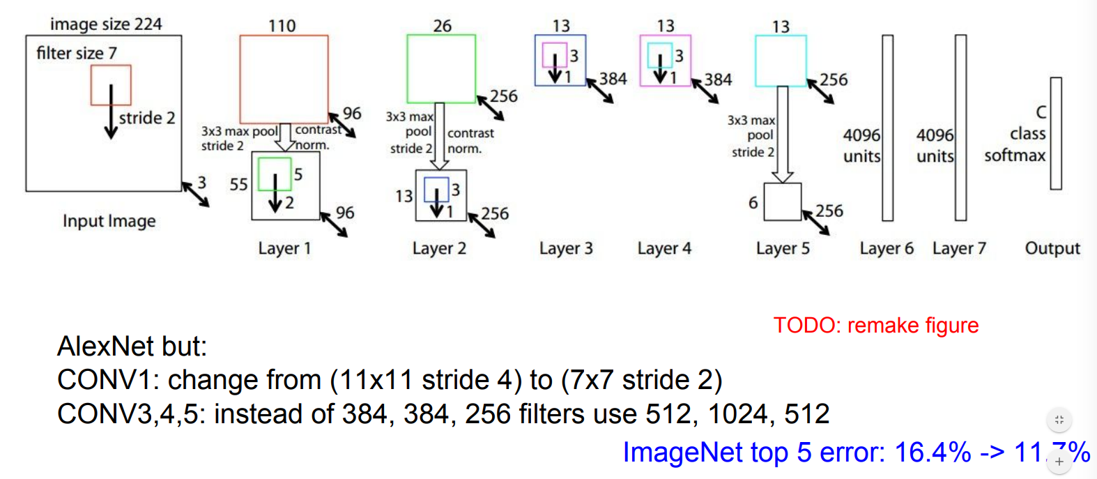
ZFNET

Architecture

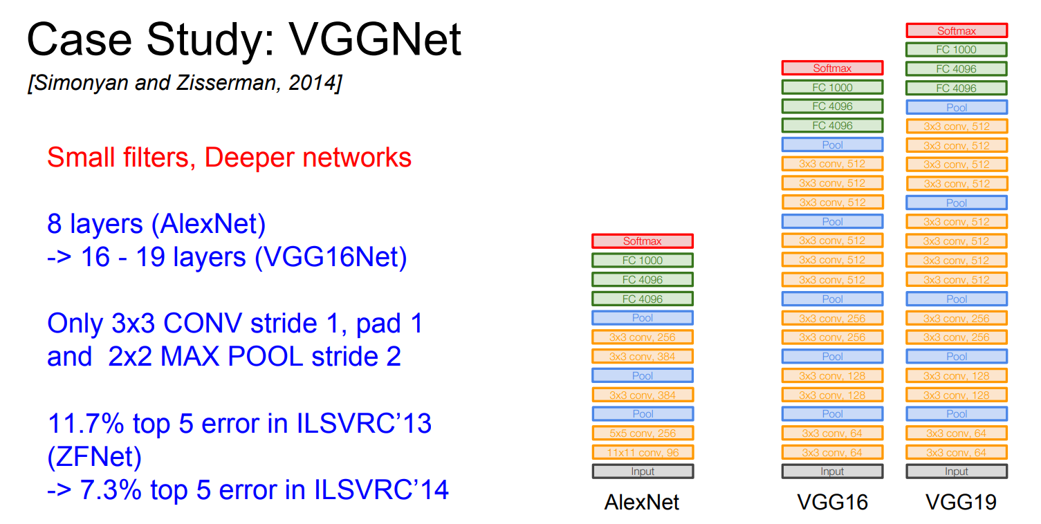
VGGNet

Architecture

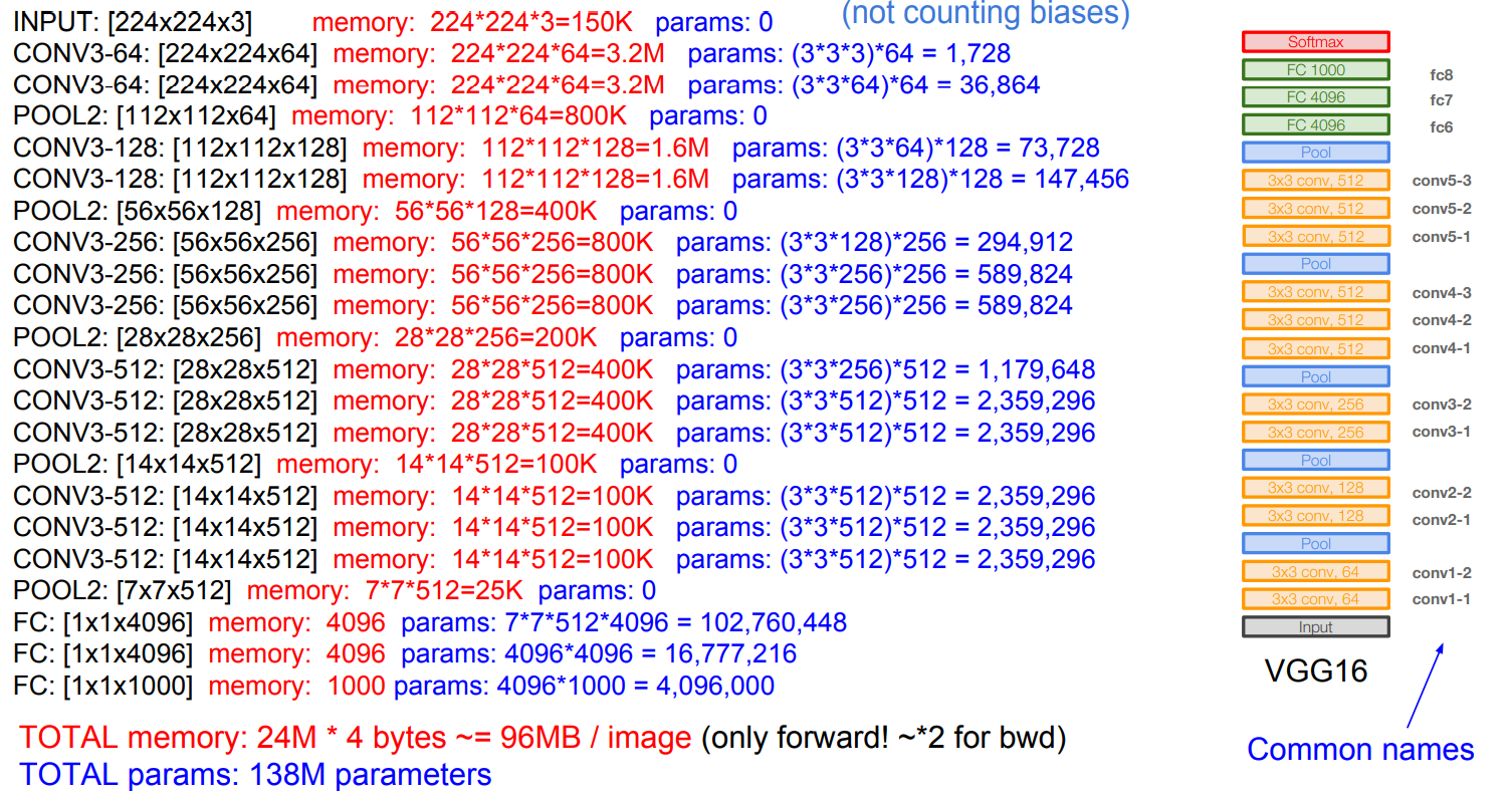
Most memory is in early CONV while most params are in late FC.

FC7 features generalize well to other tasks

Comments

1. Why use samller filters? ($3\times 3$ conv)

   Stack of three 3x3 conv (stride 1) layers has same effective receptive field as one 7x7 conv layer.

   For one $7\times 7$ layers, the filters range it can see is from 1 to 7.

   But for three layers $3\times 3$, at the first layer:

   first neuron: 1-3, second neuron: 2-4, …, firth neuron: 5-7.

   At the second layer:

   first neuron see first, second and third neurons from the first layer, resulting in seeing neurons: 1-5.

   second neuron see: 2-6; third neuron: 3-7.

   Then in the third layer:

   it sees 1-5, + 2-6, + 3-7 = 1-7.

2. What is the effective receptive field of three 3x3 conv (stride 1) layers?

   It is deeper and has more non-linearities. What is more, fewer parameters: $3 \times (3^2C^2)$ vs $7^2\times C^2$.

   ​

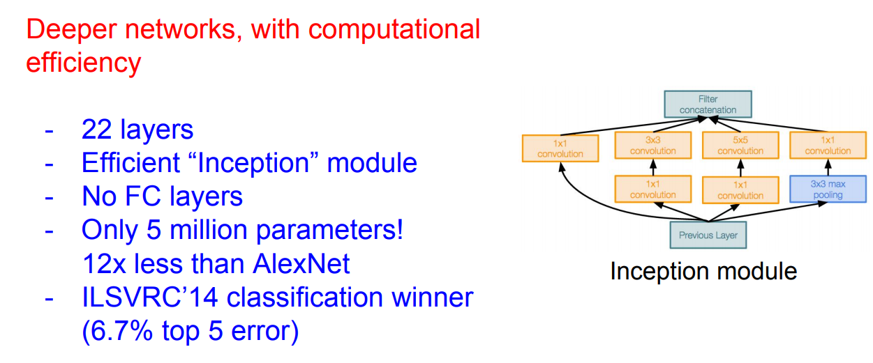
GoogLeNet

Architecture

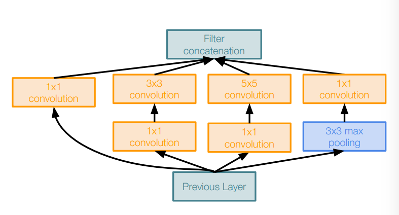
Naive Inception module

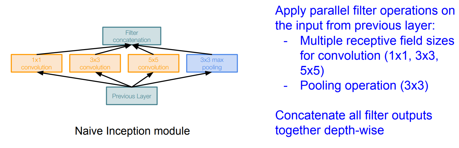
The problem:

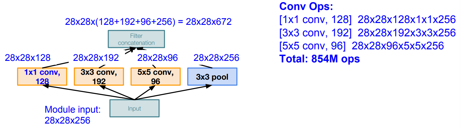
This is very expensive computation. Furthermore, Pooling layer also preserves feature depth, which means total depth after concatenation can only grow at every layer!

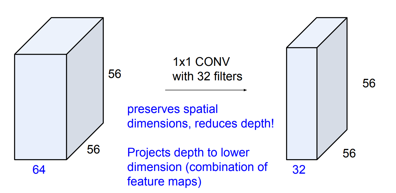
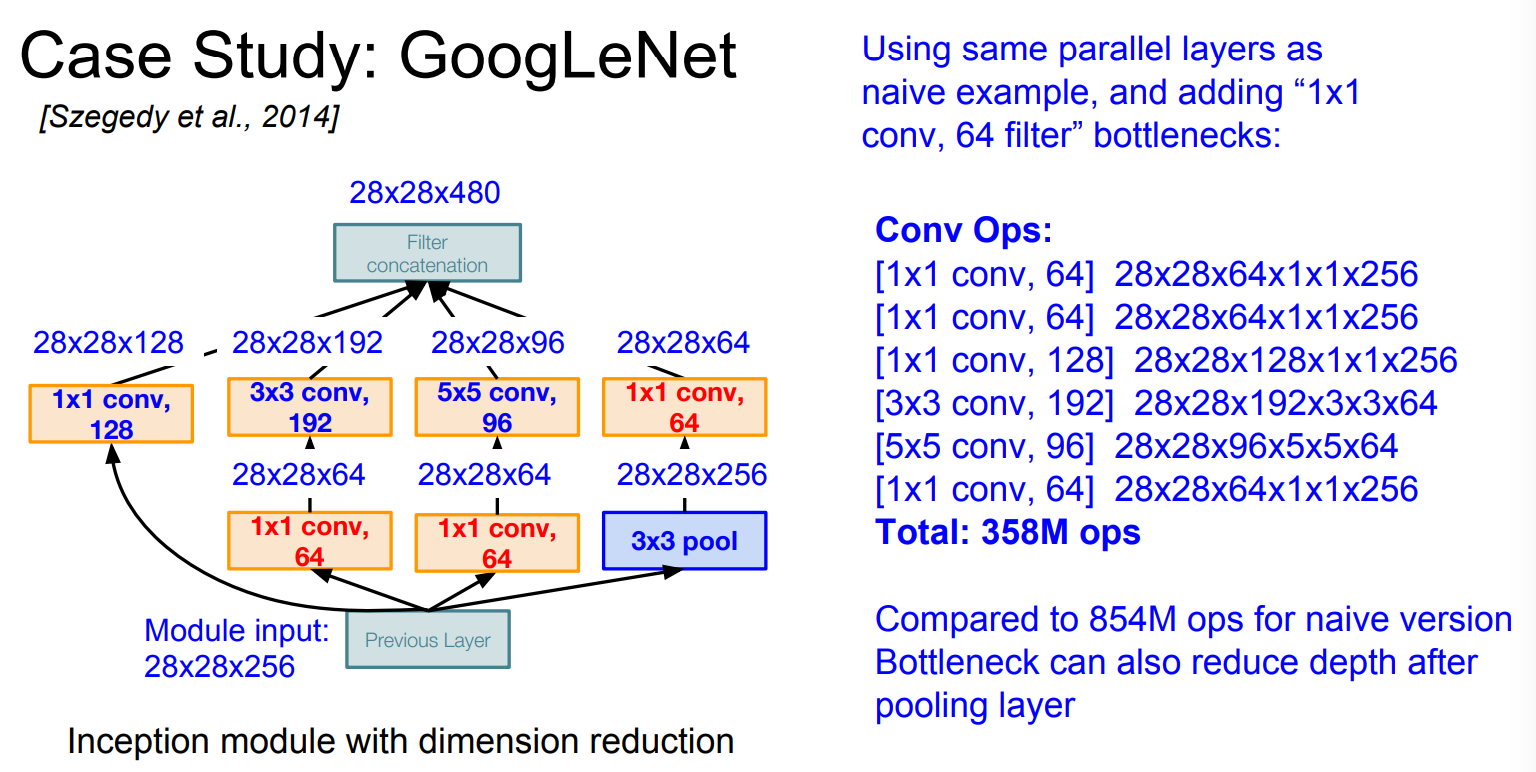
$1\times 1 \text{convolutions}$

Inception module with dimension reduction

ResNet

Architecture

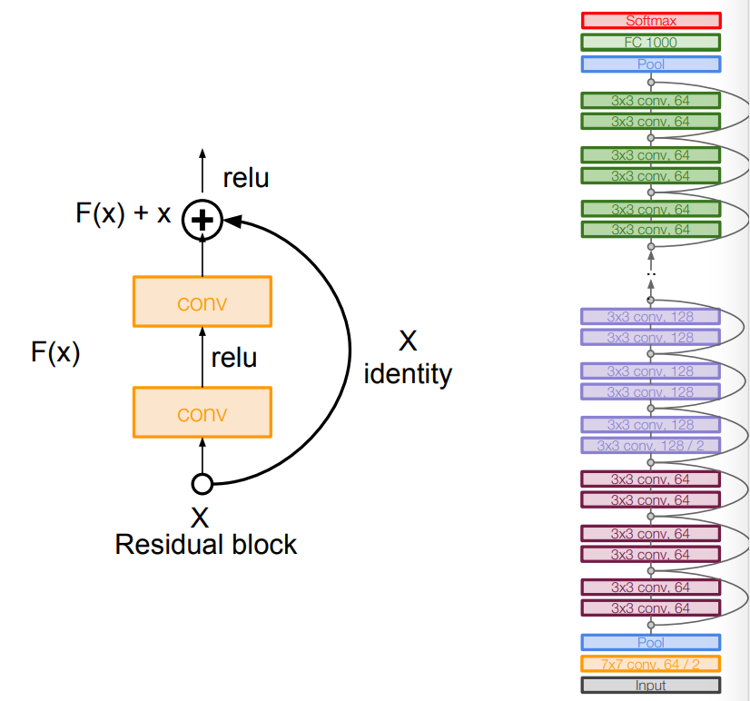
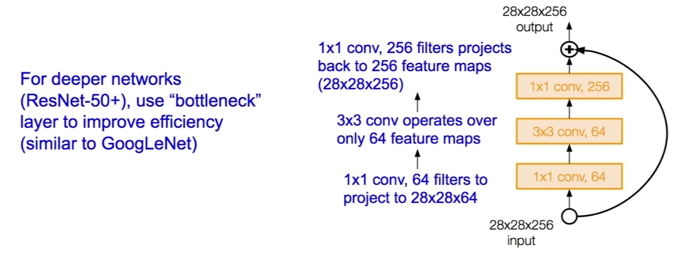
Comments

1. What happens when we continue stacking deeper layers on a “plain” convolutional neural network?

   

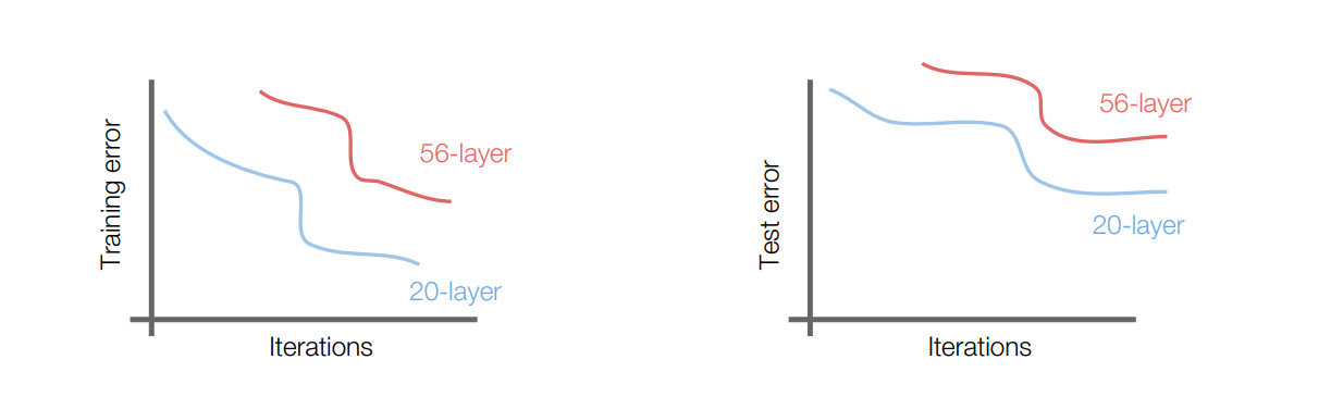
   56-layer model performs worse on both training and test error, according to the worse training loss, we can say that it is not caused by overfitting.

DenseNet

In DenseNet, each layer obtains additional inputs from all preceding layers and passes on its own feature-maps to all subsequent layers. Concatenation is used. Each layer is receiving a “collective knowledge” from all preceding layers.

SqueezeNet