Math-Linear Algebra

This is my study notes for MIT Linear Algebra.

The geometry of linear equations

The fundamental problem of linear algebra is to solve $n$ linear equations in $n$ unknowns, for example

$$\begin{aligned} 2 x-y &=0 \\-x+2 y &=3 \end{aligned}$$

Here, we are going to view this problem in three ways.

Row Picture

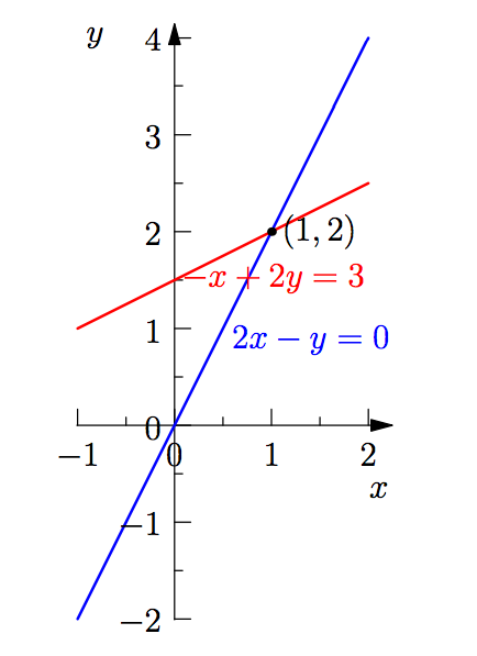
Plot the points that satisfy each equation. The intersection of the plots (if they do intersect) represents the solution to the system of equations. Looking at the following figure we see that the solution to this system of equations is $x=1,y=2$

Column Picture

In the column picture we rewrite the system of linear equations as a single
equation by turning the coefficients in the columns of the system into vectors:

$$x\left[\begin{array}{r}{2} \\ {-1}\end{array}\right]+y\left[\begin{array}{r}{-1} \\ {2}\end{array}\right]=\left[\begin{array}{l}{0} \\ {3}\end{array}\right]$$

Given two vectors $c$ and $d$ and scalars $x$ and $y$, then sum $xc+yd$ is called a linear combination of $c$ and $d$.

Matrix Picture

We can write the system of equations as a single equation by using matrices and vectors:

$$\left[\begin{array}{rr}{2} & {-1} \\ {-1} & {2}\end{array}\right]\left[\begin{array}{l}{x} \\ {y}\end{array}\right]=\left[\begin{array}{l}{0} \\ {3}\end{array}\right]$$

The matrix $A=\left[\begin{array}{rr}{2} & {-1} \\ {-1} & {2}\end{array}\right]$ is called the coefficient matrix. The vector $x=\left[\begin{array}{l}{x} \\ {y}\end{array}\right]$ is the vector of unknowns. The values on the right hand side of the equations form the vector $b$

$$Ax=b$$

Matrix Multiplication

One method to multiply a matrix $A$ by a vector $x$ is to think of $x$ as the coefficients of a linear combination of the column vectors of the matrix

$$\left[\begin{array}{ll}{2} & {5} \\ {1} & {3}\end{array}\right]\left[\begin{array}{l}{1} \\ {2}\end{array}\right]=1\left[\begin{array}{l}{2} \\ {1}\end{array}\right]+2\left[\begin{array}{l}{5} \\ {3}\end{array}\right]=\left[\begin{array}{c}{12} \\ {7}\end{array}\right]$$

or if

$$\begin{bmatrix}1&2\end{bmatrix}\left[\begin{array}{ll}{2} & {5} \\ {1} & {3}\end{array}\right]=1\begin{bmatrix}2&5\end{bmatrix}+2\begin{bmatrix}1&3\end{bmatrix}$$

Linear Independence

Given a matrix $A$, can we solve

$$Ax=b$$

for every possible vector $b$? In other words, do the linear combinations of the column vectors fill the $xy$-plane (or space, in the three dimensional case)?

If the answer is “no”, we say that A is a singular matrix. In this singular
case its column vectors are linearly dependent; all linear combinations of those vectors lie on a point or line (in two dimensions) or on a point, line or plane (in three dimensions). The combinations don’t fill the whole space.

Elimination with Matrices

Let’s look at the result matrix, i.e., the third one. For the first row, $\begin{bmatrix}1&2&1\end{bmatrix}$, it is computed by only using the first row of the second matrix, which means the elimination matrix, i.e., the first matrix, has $\begin{bmatrix}1&0&0\end{bmatrix}$ as its first row. It is the same situation with the third row. So we have elimination matrix $\begin{bmatrix}1 & 0 & 0\\ & & \\ 0&0&1\end{bmatrix}$. As for the second row, we can see that in the second matrix, its first row contributes -3 and its second row contributes 1. But there is no contribution from third row. Therefore, the elimination matrix is $\begin{bmatrix}1 & 0 & 0\\ -3& 1& 0\\ 0&0&1\end{bmatrix}$.

Inverses

If $A$ is a square matrix, the most important question you can ask about it is whether it has an inverse $A^{-1}$. If it does, then $ A^{-1}A=I=AA^{-1}$ (This is just a special form of the equation Ax = b). And we say that $A$ is invertible or nonsingular.

If A is singular – i.e. A does not have an inverse – its determinant is zero and we can find some non-zero vector x for which Ax = 0. For example:

$$\left[\begin{array}{ll}{1} & {3} \\ {2} & {6}\end{array}\right]\left[\begin{array}{r}{3} \\ {-1}\end{array}\right]=\left[\begin{array}{l}{0} \\ {0}\end{array}\right]$$

We can use the method of elimination to solve two or more linear equations at
the same time. Just augment the matrix with the whole identity matrix I:

$$\left[\begin{array}{ll|ll}{1} & {3} & {1} & {0} \\ {2} & {7} & {0} & {1}\end{array}\right] \rightarrow\left[\begin{array}{rr|rr}{1} & {3} & {1} & {0} \\ {0} & {1} & {-2} & {1}\end{array}\right] \rightarrow\left[\begin{array}{rr|rr}{1} & {0} & {7} & {-3} \\ {0} & {1} & {-2} & {1}\end{array}\right]$$ $$A^{-1}=\left[\begin{array}{rr}{7} & {-3} \\ {-2} & {1}\end{array}\right]$$

Use GaussJordan elimination on $\begin{bmatrix}U&I\end{bmatrix}$to find the upper triangular $U^{-1}$.

$$U U^{-1}=I\left[\begin{array}{ccc}{1} & {a} & {b} \\ {0} & {1} & {c} \\ {0} & {0} & {1}\end{array}\right]\left[\begin{array}{lll}{x_{1}} & {x_{2}} & {x_{3}} \\ {} & {} & {}\end{array}\right]=\left[\begin{array}{lll}{1} & {0} & {0} \\ {0} & {1} & {0} \\ {0} & {0} & {1}\end{array}\right]$$

Solution: Row reduce $\begin{bmatrix}U&I\end{bmatrix}$ to get $\begin{bmatrix}I&U^{-1}\end{bmatrix}$ as follows:

$$\left.\left[\begin{array}{cccccc}{1} & {a} & {b} & {1} & {0} & {0} \\ {0} & {1} & {c} & {0} & {1} & {0} \\ {0} & {0} & {1} & {0} & {0} & {1}\end{array}\right] \longrightarrow \begin{array}{l}{\left(R_{1}=R_{1}-a R_{2}\right)} \\ {R_{2}=R_{2}-c R_{2}}\end{array}\right)\left[\begin{array}{cccccc}{1} & {0} & {b-a c} & {1} & {-a} & {0} \\ {0} & {1} & {} & {0} & {0} & {1} & {-c} \\ {0} & {0} & {1} & {0} & {0} & {1}\end{array}\right]\\ \left(R_{1}=R_{1}-(b-a c) R_{3}\right)\left[\begin{array}{ccccc}{1} & {0} & {0} & {1} & {-a} & {a c-b} \\ {0} & {1} & {0} & {0} & {1} & {-c} \\ {0} & {0} & {1} & {0} & {0} & {1}\end{array}\right]=\left[\begin{array}{cc}{I} & {L^{-1}}\end{array}\right]$$

Permutations

Multiplication by a permutation matrix $P$ swaps the rows of a matrix; when applying the method of elimination we use permutation matrices to move zeros out of pivot positions. Our factorization $A=LU$ then becomes $PA=LU$, where $P$ is a permutation matrix which recorders any number of rows of $A$. Recall that $P^{-1}=P^{T}$, i.e., that $P^{T}P=I$.

Vector Space

We can add vectors and multiply them by numbers, which means we can discuss linear combinations of vectors. These combinations follow the rules of a vector space.

Closure

The collection of vectors with exactly two positive real valued components is not a vector space. The sum of any two vectors in that collection is again in the collection, but multiplying any vector by, say, −5, gives a vector that’s not in the collection. We say that this collection of positive vectors is closed under addition but not under multiplication.
If a collection of vectors is closed under linear combinations (i.e. under addition and multiplication by any real numbers), and if multiplication and addition behave in a reasonable way, then we call that collection a vector space.

A vector space must contain origin, i.e., it has zero vector. Because it should allow multiply by 0, or addition of negative and positive identity vectors.

A vector space is a collection of vectors which is closed under linear combinations. In other words, for any two vectors v and w in the space and any two real numbers c and d, the vector cv + dw is also in the vector space.

A plane $P$ containing $\begin{bmatrix}0\\0\\0\end{bmatrix}$ and a line $L$ containing $\begin{bmatrix}0\\0\\0\end{bmatrix}$ are both subspace of $R^3$. The union $P \cup L$ of these two subspaces is generally not a subspace, because the sum of a vector in $P$ and a vector in $L$ is probably not contained in $P \cup L$. The intersection $S \cap T$ of two subspaces $S$ and $T$ is a subspace. To prove this, use the fact that both $S$ and $T$ are closed under linear combinations to show that their intersection is closed under linear combinations.

Subspace

A vector space that is contained inside of another vector space is called a subspace of that space. For example, take any non-zero vector $v$ in $R^2$. Then the set of all vectors $cv$, where $c$ is a real number, forms a subspace of $R^2 $. This collection of vectors describes a line through $\begin{bmatrix}0\\0\end{bmatrix}$ in $R^2$ and is closed under addition.

A line in $R^2$ that does not pass through the origin is not a subspace of $R^2$. Multiplying any vector on that line by 0 gives the zero vector, whcih does not line on the line. Every subspace must contain the zero vector because vector spaces are closed under multiplication.

The subspace of $R^2$ are:

1. all of $R^2$
2. any line through $\begin{bmatrix}0\\0\end{bmatrix}$ and
3. the zero vector alone

The subspace of $R^3$ are:

1. all of $R^3$
2. any plane through the origin
3. any line through the origin, and
4. the zero vector alone

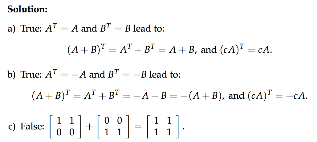
First of all, here $M$ is a set containing all symmetric matrices. According to the definition of subspace, as long as the vectors in that set is closed, then it is a space. So, we use two symmetric matrix $A$ and $B$ and prove whether $(A+B)$ and $cA$ are symmetric.

Column space

Given a matrix $A$ with columns in $R^3$, these columns and all their linear combinations form a subspace of $R^3$. This is the column space $C(A)$. If $A=\begin{bmatrix}1&2\\2&3\\4&1\end{bmatrix}$, the column space of $A$ is the plane through the origin in $R^3$ containing $A=\begin{bmatrix}1\\2\\4\end{bmatrix}$ and $A=\begin{bmatrix}2\\3\\1\end{bmatrix}$

In a nutshell, the column space of a matrix $A$ is the vector space made up of all linear combinations of the columns of $A$.

Solving $Ax=b$

Given a matrix $A$, for what vectors $b$ does $Ax=b$ have a solution?

$$\text { Let } A=\left[\begin{array}{lll}{1} & {1} & {2} \\ {2} & {1} & {3} \\ {3} & {1} & {4} \\ {4} & {1} & {5}\end{array}\right]$$

Then $Ax = b$ does not have a solution for every choice of b because solving $Ax = b$ is equivalent to solving four linear equations in three unknowns. If there is a solution to $Ax = b$, then $b$ must be a linear combination of the columns of A. Only three columns cannot fill the entire four dimensional vector space – some vectors b cannot be expressed as linear combinations of columns of A.

Big question: what $b$’s allow $Ax=b$ to be solved?

The system of linear equations $Ax=b$ is solvable exactly when b is a vector in the column space of $A$.

For our example matrix $A$, what can we say about the column space of $A$? Are the columns of $A$ independent? In other words, does each column contribute something new to the subspace? The third column of $A$ is the sum of the first two columns, so does not add anything to the subspace. The column space of our matrix $A$ is a two dimensional subspace of $R^4$.

Nullspace of Matrix

The nullspace of a matrix $A$ is the collection of all solutions $x=\begin{bmatrix}x_1 \\x_2 \\x_3 \end{bmatrix}$ to the equation $Ax=0$. The column space of the matrix in our example was a subpace of $R^4$. The nullspace of $A$ is a subspace of $R^3$. To see that it’s a vector space, check that any sum or multiple of solutions to $Ax=0$ is a also solution: $A(x_1+x_2)=Ax_1+Ax_2=0+0$ and $A(cx)=cAx=c(0)$.

In the example,

$$\left[\begin{array}{lll}{1} & {1} & {2} \\ {2} & {1} & {3} \\ {3} & {1} & {4} \\ {4} & {1} & {5}\end{array}\right]\left[\begin{array}{l}{x_{1}} \\ {x_{2}} \\ {x_{3}}\end{array}\right]=\left[\begin{array}{l}{0} \\ {0} \\ {0} \\ {0}\end{array}\right]$$

the nullspace $N(A)$ consists of all multiples of $\begin{bmatrix} 1 \\ 1 \\ -1 \end{bmatrix}$. column 1 plus column 2 minus column 3 equals the zero vector. This nullspace is a line in $R^3$.

Other values of b

The solutions to the equations:

$$\left[\begin{array}{lll}{1} & {1} & {2} \\ {2} & {1} & {3} \\ {3} & {1} & {4} \\ {4} & {1} & {5}\end{array}\right]\left[\begin{array}{l}{x_{1}} \\ {x_{2}} \\ {x_{3}}\end{array}\right]=\left[\begin{array}{l}{1} \\ {2} \\ {3} \\ {4}\end{array}\right]$$

do not form a subspace. The zero vector is not a solution to this equation. The set of solutions forms a line in $R^3$ that passes through the points $\begin{bmatrix}1 \\0 \\0 \end{bmatrix}$ and $\begin{bmatrix}0 \\ -1 \\1 \end{bmatrix}$ but not $\begin{bmatrix}0 \\0 \\0 \end{bmatrix}$

computing the nullspace

Suppose

$$A=\left[\begin{array}{llll}{1} & {2} & {2} & {2} \\ {2} & {4} & {6} & {8} \\ {3} & {6} & {8} & {10}\end{array}\right]$$

Our algorithm for computing the nullspace of this matrix uses the method of elimination, despite the fact that A is not invertible. We don’t need to use an augmented matrix because the right side (the vector b) is 0 in this computation.

The first step of elimination gives us:

$$A=\left[\begin{array}{llll}{1} & {2} & {2} & {2} \\ {2} & {4} & {6} & {8} \\ {3} & {6} & {8} & {10}\end{array}\right] \quad \longrightarrow \quad\left[\begin{array}{llll}{1} & {2} & {2} & {2} \\ {0} & {0} & {2} & {4} \\ {0} & {0} & {2} & {4}\end{array}\right]$$

We don’t find a pivot in the second column, so our next pivot is the 2 in the third column of the second row:

$$\left[\begin{array}{llll}{1} & {2} & {2} & {2} \\ {0} & {0} & {2} & {4} \\ {0} & {0} & {2} & {4}\end{array}\right] \quad \longrightarrow \quad\left[\begin{array}{llll}{1} & {2} & {2} & {2} \\ {0} & {0} & {2} & {4} \\ {0} & {0} & {0} & {0}\end{array}\right]=U$$

The matrix U is in echelon (staircase) form. The third row is zero because row 3 was a linear combination of rows 1 and 2; it was eliminated. The rank of a matrix A equals the number of pivots it has. In this example, the rank of A (and of U) is 2.

special solutions

Once we’ve found U we can use back-substitution to find the solutions x to the equation Ux = 0. In our example, columns 1 and 3 are pivot columns containing pivots, and columns 2 and 4 are free columns. We can assign any value to x2 and x4; we call these free variables. Suppose x2 = 1 and x4 = 0. Then:

$$2x_3+4x_4=0 => x_3=0$$

and

$$x_1+2x_2+2x_3+2x_4=0 =>x_1=-2$$

so one solution is $x=\begin{bmatrix}-2\\1\\0\\0\end{bmatrix}$. Any multiple of this vector is in the nullspace.

Letting a different free variable equal 1 and setting the other free variables equal to 0 gives us other vectors in the nullspace. For example:

$$x=\begin{bmatrix}2\\0\\-2\\1\end{bmatrix}$$

The rank $r$ of A equals the number of pivot columns, so the number of free columns is $n − r$: the number of columns (variables) minus the number of pivot columns. This equals the number of special solution vectors and the dimension of the nullspace.

Reduced row echelon form

By continuing to use the method of elimination we can convert U to a matrix R in reduced row echelon form (rref form), with pivots equal to 1 and zeros above and below the pivots.

$$U=\left[\begin{array}{llll}{1} & {2} & {2} & {2} \\ {0} & {0} & {2} & {4} \\ {0} & {0} & {0} & {0}\end{array}\right] \rightarrow\left[\begin{array}{rrrr}{1} & {2} & {0} & {-2} \\ {0} & {0} & {2} & {4} \\ {0} & {0} & {0} & {0}\end{array}\right] \rightarrow\left[\begin{array}{rrrr}{1} & {2} & {0} & {-2} \\ {0} & {0} & {1} & {2} \\ {0} & {0} & {0} & {0}\end{array}\right]=R$$

By exchanging some columns, R can be rewritten with a copy of the identity matrix in the upper left corner, possibly followed by some free columns on the right. If some rows of A are linearly dependent, the lower rows of the matrix R will be filled with zeros:

$$R=\left[\begin{array}{cc}{I} & {F} \\ {0} & {0}\end{array}\right]$$

(Here I is an r by r square matrix.)

If N is a nullspace matrix $N=\begin{bmatrix}-F\\I\end{bmatrix}$ then $RN=0$. (Here I is an n − r by n − r square matrix and 0 is an m by n − r matrix.) The columns of N are the special solutions.

In this example, we have $-F=\begin{bmatrix}0&-2\-1&-2\\1&0\\0&1\end{bmatrix}$. So the special solutions to $Ax=0$ are:

$$\left[\begin{array}{r}{0} \\ {-1 } \\ {1} \\ {0}\end{array}\right] \text { and }\left[\begin{array}{r}{-2 } \\ {-2} \\ {0} \\ {1}\end{array}\right]$$

Solving Ax=b

Solvability conditions on b

when does $Ax=b$ have solutions and how can we describe those solutions?

We again use the example:

$$A=\left[\begin{array}{llll}{1} & {2} & {2} & {2} \\ {2} & {4} & {6} & {8} \\ {3} & {6} & {8} & {10}\end{array}\right]$$

The third row of A is the sum of its first and second rows, so we know that if Ax = b the third component of b equals the sum of its first and second components. If b does not satisfy b3 = b1 + b2 the system has no solution. If a combination of the rows of A gives the zero row, then the same combination of the entries of b must equal zero.

One way to find out whether Ax = b is solvable is to use elimination on the augmented matrix. If a row of A is completely eliminated, so is the corresponding entry in b. In our example, row 3 of A is completely eliminated:

$$\left[\begin{array}{ccccc}{1} & {2} & {2} & {2} & {b_{1}} \\ {2} & {4} & {6} & {8} & {b_{2}} \\ {3} & {6} & {8} & {10} & {b_{3}}\end{array}\right] \rightarrow \cdots \rightarrow\left[\begin{array}{ccccc}{1} & {2} & {2} & {2} & {b_{1}} \\ {0} & {0} & {2} & {4} & {b_{2}-2 b_{1}} \\ {0} & {0} & {0} & {0} & {b_{3}-b_{2}-b_{1}}\end{array}\right]$$

If $Ax=b$ has a solution, then $b_3-b_2-b_1=0$. For example, we could choose $b=\begin{bmatrix}1\\5\\6\end{bmatrix}$. From an earlier lecture, we know that Ax = b is solvable exactly when b is in the column space C(A). We have these two conditions on b; in fact they are equivalent.

Complete solution

In order to find all solutions to Ax = b we first check that the equation is solvable, then find a particular solution. We get the complete solution of the equation by adding the particular solution to all the vectors in the nullspace.

A particular solution

One way to find a particular solution to the equation Ax = b is to set all free variables to zero, then solve for the pivot variables.

For our example matrix $A$, we let $x_2=x_4=0$ to get the system of equations:

$$\begin{aligned} x_{1}+2 x_{3} &=1 \\ 2 x_{3} &=3 \end{aligned}$$

which has the solution $x_3=\frac{3}{2}, x_1=-2$. Our particular solution is:

$$\mathbf{x}_{p}=\left[\begin{array}{r}{-2} \\ {0} \\ {3 / 2} \\ {0}\end{array}\right]$$

Combined with the nullspace

The general solution to $Ax=b$ is given by $X_{complete}=x_p+x_n$, where $x_n$ is a generic vector in the nullspace. To see this, we add $Ax_p=b$ to $Ax_n=0$ and get $A(x_p+x_n)=b$ for every vector in the nullspace.

We know that the nullspace of $A$ is the collection of all combinations of the special solutions $\begin{bmatrix}-2\\1\\0\\0\end{bmatrix}$ and $\begin{bmatrix}2\\0\-2\\1\end{bmatrix}$. So the complete solution to the equation $Ax=\begin{bmatrix}1\\5\\6\end{bmatrix}$ is:

$$\mathbf{x}_{\text {complete }}=\left[\begin{array}{r}{-2} \\ {0} \\ {3 / 2} \\ {0}\end{array}\right]+c_1\left[\begin{array}{r}{-2} \\ {1} \\ {0} \\ {0}\end{array}\right]+c_{2}\left[\begin{array}{r}{2} \\ {0} \\ {-2} \\ {1}\end{array}\right]$$

where $c_1$ and $c_2$ are real numbers.

The nullspace of $A$ is a two dimensional subspace of $R^4$, and the solutions to the equation $Ax=b$ form a plane parallel to that through $x_p=\left[\begin{array}{r}{-2} \\ {0} \\ {3 / 2} \\ {0}\end{array}\right]$.

Rank

The rank of a matrix equals the number of pivots of that matrix. If $A$ is an $m$ by $n$ matrix of rank $r$, we know that $r\le m$ and $r\le n$.

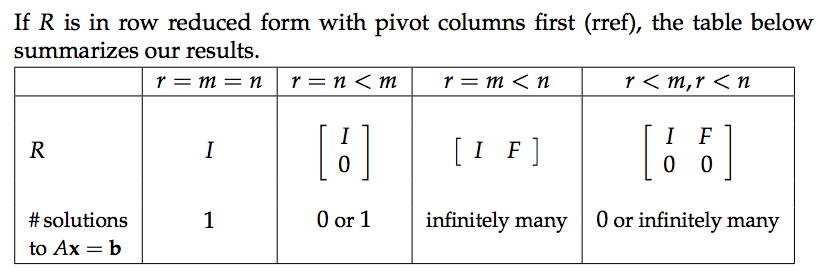
Full column rank

If $r=n$, then the nullspace has dimension $n-r=0$ and contains only zero vector. There are no free variables or special solutions.

Since there are going to have zero rows after row reduction, so the combinations of $b$ should be zero too. In this case, $Ax=b$ has a solution and it is unique. Otherwise, there is no solution.

The row reduced echelon form of the matrix will look like $R=\begin{bmatrix}I\\0\end{bmatrix}$.

Full row rank

If $r=m$, then the reduced matrix $R=\begin{bmatrix}I&F\end{bmatrix}$ has no rows of zeros and so there are no requirements for the entries of $b$ to satisfy. The equation $Ax=b$ is solvable for every $b$. There are $n-m$ free variables, so there are $n-m$ special solutions to $Ax=0$

Full row and column rank

If $r=m=n$ is the number of pivots of $A$, then $A$ is an invertible square matrix and $R$ is the identity matrix. The nullspace has dimension zero and $Ax=b$ has a unique solution for every $b$.

Summary

Linear independence

Suppose $A$ is $m$ by $n$ with $m < n$. Then there are non-zero solutions to $Ax=0$. This is a equation with more unknowns than equations. So there will be free variables. A combination of the columns is zero, so the columns of this $A$ are dependent.

We say vectors $x_1,x_2,…x_n$ are linearly indepent if $c_1x_1+c_2x_2+…+c_nx_n=0$ only when $c_1,c_2,…,c_n$ are all 0. When those vectors are the columns of $A$, the only solution to $Ax=0$ is $x=0$.

Two vectors are independent if they do not lie on the same line. Three vectors are independent if they do npt lie in the same plane. Thinking of $Ax$ as a linear combination of the column vctors of $A$, we see that the column vectors of $A$ are independent exactly when the nullspace of $A$ contains only the zero vector.

Say we have three vectors in the $x-y$ plane. So each vector is a $\begin{bmatrix}a\\b \end{bmatrix}$. But we have three unknowns, meaning there must be free variables according to the first paragraph.

If the columns of $A$ are independent then all columns are pivot columns, the rank of $A$ is $n$, and there are no free variables. If the columns of $A$ are dependent then the rank of $A$ is less than $n$ and there are free variables.

Spanning a space

Vectors $v_1,v_2,…,v_k$ span a space when the space consists of all combinations of those vectors. For example, the column vectors of $A$ span the column space of $A$. If vectors $v_1,v_2,…,v_k$ span a space $S$, then $S$ is the smalles space containing those vectors.

Basis and dimension

A basis for a vector space is a sequence of vectors $v_1,v_2,…,v_d$ with two properties:

• $v_1,v_2,…,v_d$ are independent
• $v_1,v_2,…,v_d$ span the vector space

Example $R^3$:

One basis for $R^3$ is $\left\{\left[\begin{array}{l}{1} \\ {0} \\ {0}\end{array}\right],\left[\begin{array}{l}{0} \\ {1} \\ {0}\end{array}\right],\left[\begin{array}{l}{0} \\ {0} \\ {1}\end{array}\right]\right\}$.However, the vectors $\begin{bmatrix}1\\1\\2\end{bmatrix}$, $\begin{bmatrix}2\\2\\5\end{bmatrix}$ and $\begin{bmatrix}3\\3\\8\end{bmatrix}$ do not form a basis for $R^3$ because the third vector is in the space of the first two vectors. In general, for a square matrix, i.e., $n$ vectors in $R^n$, form a basis if they are the column vectors of an invertible matrix.

The vectors $\begin{bmatrix}1\\1\\2\end{bmatrix}$ and $\begin{bmatrix}2\\2\\5\end{bmatrix}$ span a plane in $R^3$ but they cannot form a basis for $R^3$. However, they form a basis of column space for matrix $\begin{bmatrix}1 ,2,3\\1,2,3\\2,5,8\end{bmatrix}$.

Given a space, every basis for that space has the same number of vectors; that number is the dimension of the space, So there are exactly $n$ vectors in every basis for $R^n$.

Bases of a column space and nullspace

Suppose:

$$A=\left[\begin{array}{llll}{1} & {2} & {3} & {1} \\ {1} & {1} & {2} & {1} \\ {1} & {2} & {3} & {1}\end{array}\right]$$

By definition, the four column vectors of $A$ span the column space of $A$. The third and fourth column vectors are dependent on the first and second, and the first two columns are independent. Therefore, the first two column vectors are the pivot columns. They form a basis for the column space $C(A)$. The matrix has rank 2.

$$\text{rank}(A)=\text{number of pivot columns of }A=\text{dimension of } C(A)$$

The column vectors of this $A$ are not independent, so the nullspace $N(A)$ contains more than just zero vectors. Because the third column is the sum of the first two, we know that the vector $\begin{bmatrix}-1\\ -1\\1\\0\end{bmatrix}$ is in the nullspace. Similarly, $\begin{bmatrix}-1\\0\\0\\ -1\end{bmatrix}$ is also in $N(A)$. These are the two special solutions to $Ax=0$.

$$\text{dimension of }N(A)=\text{number of free variables}=n-r$$

so we know that the dimension of $N(A)$ is 4-2=2. These two special solutions form a basis for the nullspace.

The Four Fundamental Subspaces

Any $m$ by $n$ matrix $A$ determines four subspaces

column space $C(A)$: consists of all combinations of the columns of $A$ and is a vector space in $R^m$.

The $r$ pivot columns form a basis for $C(A)$: $\text{dim} C(A)=r$.

nullspace $N(A)$ consists of all solutions $x$ of the equation $Ax=0$ and lies in $R^n$.

The special solutions to $Ax=0$ correspond to free variables and form a basis for $N(A)$. An $m$ by $n$ matrix has $n-r$ free variables: $\text{dim} N(A)=n-r$.

row space $C(A^T)$, the combinations of the row vectors of $A$ form a subspace of $R^n$. We equate this with $C(A^T)$, the column space of the transpose of $A$.

We could perform row reduction on $A^T$, but insted we make use of $R$, the row reduced echelon form of $A$.

$$A=\left[\begin{array}{llll}{1} & {2} & {3} & {1} \\ {1} & {1} & {2} & {1} \\ {1} & {2} & {3} & {1}\end{array}\right] \rightarrow \cdots \rightarrow\left[\begin{array}{llll}{1} & {0} & {1} & {1} \\ {0} & {1} & {1} & {0} \\ {0} & {0} & {0} & {0}\end{array}\right]=\left[\begin{array}{ll}{I} & {F} \\ {0} & {0}\end{array}\right]=R$$

Although the column spaces of $A$ and $R$ are different, the row space of $R$ is the same as the row space of $A$. The rows of $R$ are combinations of the rows of $A$, and because reduction is reversible the rows of $A$ are combinations of the rows of $R$. The first $r$ rows of $R$ are the echelon basis for the row space of $A$: $\text{dim}C(A^T)=r$. In this exampe, there is a basis consisting of two vectors: $\begin{bmatrix}1\ 0\ 1\ 1\end{bmatrix}$ and $\begin{bmatrix}0\ 1\ 1\ 0\end{bmatrix}$.

left nullspace, $N(A^T)$, is a subspace of $R^m$.

The matrix $A^T$ has $m$ columns. We just saw that $r$ is the rank of $A^T$, so the number of free columns of $A^T$ must be $m-r$: $\text{dim}N(A^T)=m-r$. The left nullspace is the collection of vectors $y$ for which $A^Ty=0$. Equivalently, $y^T A=0$; here $y$ and 0 are row vectors. We say left nullspace because $y^T$ is on the left of $A$ in this equation. To find a basis for the left nullspace we reduce an augmented version of $A$:

$$\left[\begin{array}{ll}{A_{m \times n}} & {I_{m \times n}}\end{array}\right] \longrightarrow\left[\begin{array}{ll}{R_{m \times n}} & {E_{m \times n}}\end{array}\right]$$

From this we get the matrix $E$ for which $EA=R$. (If $A$ is a square, invertible matrix then $E=A^{-1}$). In our example,

$$E A=\left[\begin{array}{rrr}{-1} & {2} & {0} \\ {1} & {-1} & {0} \\ {-1} & {0} & {1}\end{array}\right]\left[\begin{array}{llll}{1} & {2} & {3} & {1} \\ {1} & {1} & {2} & {1} \\ {1} & {2} & {3} & {1}\end{array}\right]=\left[\begin{array}{llll}{1} & {0} & {1} & {1} \\ {0} & {1} & {1} & {0} \\ {0} & {0} & {0} & {0}\end{array}\right]=R$$

the bottom $m-r$ rows of $E$ describe linear dependencies of rows of $A$, because the bottome $m-r$ rows of $R$ are zero. Here $m-r=1$, the bottom $m-r$ rows of $E$ satisfy the equation $y^TA=0$ and form a basis for the left nullspace of $A$.

Rank one matrices

The rank of a matrix is the dimension of its column (or row) space. The matrix

$$A=\left[\begin{array}{ccc}{1} & {4} & {5} \\ {2} & {8} & {10}\end{array}\right]$$

has rank 1 because each of its columns is a multiple of the first column.

$$A=\left[\begin{array}{l}{1} \\ {2}\end{array}\right]\left[\begin{array}{lll}{1} & {4} & {5}\end{array}\right]$$

Every rank 1 matrix $A$ can be written $A=UV^T$, where $U$ and $V$ are column vectors. We’ll use rank 1 matrices as building blocks for more complex matrices.

Orthogonal&Projection

If two vectors are orthogonal, they form a right triangle whose hypotenuse is the sum of the vectors. Thus, we can use the Pythagorean theorem to prove that the dot product $x^Ty=y^Tx$ is zero exactly when $x$ and $y$ are orthogonal. The length squared $||x||^2$ equals $x^Tx$. Note that all vectors are orthogonal to the zero vector.

Subspace S is orthogonal to subspace T means: every vector in S is orthogonal to every vector in T.

Nullspace is perpendicular to row space

The row space of a matrix is orthogonal to the nullspace, because Ax = 0 means the dot product of x with each row of A is 0. Then the product of x with any combination of rows of A must be 0. The column space is orthogonal to the left nullspace of A because the row
space of $A^T$ is perpendicular to the nullspace of $A^T$.

$A^TA$ is square and symmetric. In fact:

$$\begin{aligned} N\left(A^{T} A\right) &=N(A) \\ \text { rank of } A^{T} A &=\operatorname{rank} \text { of } A \end{aligned}$$

We conclude that $A^TA$ is invertible exactly when A has independent columns.

Projection

If we have a vector $b$ and a line determined by a vector $a$, how do we find the point on the line that is closest to $b$?

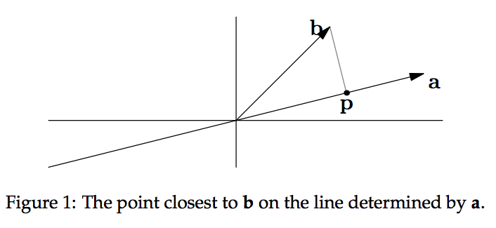
We can see from Figure 1 that this closest point $p$ is at the intersection formed by a line through $b$ that is orthogonal to $a$. If we think of $p$ as an approximation of $b$, then the length of $e=b-p$ is the error in that approximation. Since $p$ lies on the line through $a$, we know $p=xa$ for some number $x$. We also know that $a$ is perpendicular to $e=b-xa$:

$$a^T(b-ax)=0\\ a^Txa=a^Tb\\ x=\frac{a^Tb}{a^Ta}$$

Remember that $a^Ta$ is a number. $p=ax=a\frac{a^Tb}{a^Ta}$. Doubling $b$ doubles $p$. Doubling $a$ does not affect $p$.

Projection matrix

We’d like to write this projection in terms of a projection matrix $P:p=Pb$.

$$p=ax=a\frac{a^Tb}{a^Ta}$$

so the matrix is:

$$P=\frac{aa^T}{a^Ta}$$

Note that $aa^T$ is a matrix, not a number. Since for any $b$, $Pb$ lines on the line $a$, thus, the column space of $P$ is spanned by $a$. The rank of $P$ is 1. $P$ is symmetric. $P^2b=Pb$ because the projection of a vector already on the line through $a$ is just that vector. In general, projection matrices have the properties:

$$P^T=P \ \text{and} \ P^2=P$$

why projection

As we know, the equation $Ax=b$ may have no solution. The vector $Ax$ is always in the column space of $A$, and $b$ is unlikely to be in the column space. So we project $b$ onto a vector $p$ in the column space of $A$ and solve $A \hat x=p$.

Projection in higher dimensions

In $R^3$,how do we project a vector $b$ onto the closest point $p$ in a plane? If $a_1$ and $a_2$ form a basis for the plane, then that plane is the column space of the matrix $A=\begin{bmatrix}a_1 \ a_2 \end{bmatrix}$. We know that $p=\hat x_1 a_1+\hat x_2a_2=A \hat x$. We want to find $\hat x$. There are many ways to show that $e=b-p=b-A \hat x$ is orthogonal to the planewe are projecting onto, after which we can use the fact that $e$ is perpendicular to $a_1$ and $a_2$:

$$\mathbf{a}_{1}^{T}(\mathbf{b}-A \hat{\mathbf{x}})=0 \quad \text { and } \quad \mathbf{a}_{2}^{T}(\mathbf{b}-A \hat{\mathbf{x}})=0$$

In matrix form, $A^T(b-A \hat x)=0$. When we were projecting onto a line, $A$ only had one column and so this equation looked like: $a^T (b-xa)=0$. Note that $e=b-A \hat x$ is in the nullspace of $A^T$ and so is in the left nullspace of $A$. We know that everything in the left nullspace of $A$ is perpendicular to the column space of $A$, so this is another confirmation that our calculation are correct.

We can rewrite the equation $A^T(b-A \hat x)=0$ as:

$$A^{T} A \hat{\mathbf{x}}=A^{T} \mathbf{b}$$

When projecting onto a line, $A^TA$ was just a number; now it is a square matrix. So insted of dividing by $a^Ta$ we now have to multiply by $(A^TA)^{-1}$, in $n$ dimensions:

$$\begin{aligned} \hat{\mathbf{x}} &=\left(A^{T} A\right)^{-1} A^{T} \mathbf{b} \\ \mathbf{p}=A \hat{\mathbf{x}} &=A\left(A^{T} A\right)^{-1} A^{T} \mathbf{b} \\ P &=A\left(A^{T} A\right)^{-1} A^{T} \end{aligned}$$

It is tempting to try to simplify these expressions, but if $A$ isn’t a square matrix we can’t say that $(A^TA)^{-1}=A^{-1}(A^T)^{-1}$. If $A$ does happen to be a square and invertible matrix, then its column space is the whole space and contains $b$. In this case $P$ is the identity, as we find when we simplify. It is still true that:

$$P^T=P \ \text{and} \ P^2=P$$

If $b$ is perpendicular to the column space, then it’s in the left nullspace $N(A^T)$ of $A$ and $Pb=0$.

According to b perpendicular to the column space of $A$, we have $A^Tb=0$. And we have $Pb$ as follows:

$$Pb = A(A^TA)^{-1}A^T b= A(A^TA)^{-1}\cdot 0 = 0$$

If $b$ is in the column space, then $b=Ax$ for some $x$, and $Pb=b$.

Similarly, $Pb = A(A^TA)^{-1}A^T b$. Substitute $b$ with $Ax$, we have $Pb=A(A^TA)^{-1}A^T Ax$. $A^TA$ are cancelled by its inverse matrix $(A^TA)^{-1}$ and results in $I$. So we have $Pb=Ax=b$.

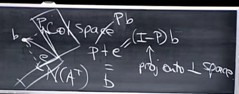
For a typical vector $b$, it will have a component $p$ in the column space and a component $e$ perpendicular to the column space, which menas $e$ is in the left nullspace. The matrix projecting $b$ onto $N(A^T)$ is $I-P$:

$$\begin{array}{l}{\mathbf{e}=\mathbf{b}-\mathbf{p}} \\ {\mathbf{e}=(I-P) \mathbf{b}}\end{array}$$

Naturally, $I-P$ has all the properties of a projection matrix.

Least Squares

Suppose we’re given a collection of data points $(t,b)$:

$$\{(1,1),(2,2),(3,2)\}$$

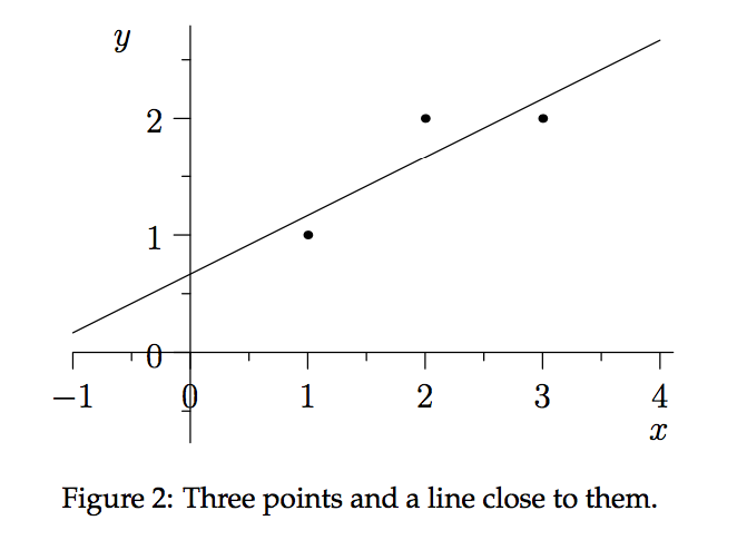
and we want to find the closest line $b=C+Dt$ to that collection. By “closest” line we mean one that minimizes the error represented by the distance from the points to the line. We measure that error by adding up the squares of these distances. In other words, we want to minimize $||Ax-b||^2=||e||^2$.

If the line went through all three points, we’d have:

$$C+D=1\\ C+2D=2\\ C+3D=2$$

which is equivalent to:

$$\left[\begin{array}{ll}{1} & {1} \\ {1} & {2} \\ {1} & {3}\end{array}\right] \quad\left[\begin{array}{l}{C} \\ {D}\end{array}\right]=\left[\begin{array}{l}{1} \\ {2} \\ {2} \\ {b}\end{array}\right]$$

There are two ways of viewing this. In the space of the line we’re trying to find, $e_1,e_2$ and $e_3$ are the vertical distances from the data points to the line. The components $p_1, p_2$ and $p_3$ are the values of $C+Dt$ near each data point; $p \approx b$.

In the other view we have a vector $b$ in $R^3$, its projection $p$ onto the column space of $A$, and its projection $e$ onto $N(A^T)$. We will now find $\hat x=\begin{bmatrix}\hat C \ \hat D \end{bmatrix}$ and $p$. We know:

$$A^TA \hat x=A^T b\\ \left[\begin{array}{cc}{3} & {6} \\ {6} & {14}\end{array}\right]\left[\begin{array}{c}{\hat{\mathrm{C}}} \\ {\hat{D}}\end{array}\right]=\left[\begin{array}{c}{5} \\ {11}\end{array}\right]$$

From this equation we get the normal equations:

$$\begin{aligned} 3 \hat C+6 \hat D &=5 \\ 6 \hat{C}+14 \hat D &=11 \end{aligned}$$

We solve these to find $\hat D=\frac{1}{2}$ and $\hat C=\frac{2}{3}$.

By using these closest line $b=\frac{2}{3}+\frac{1}{2}t$, we can find the $p$ by plugging three points into the line:

$$p=\begin{bmatrix}\frac{2}{3}+\frac{1}{2}*1 \\ \frac{2}{3}+\frac{1}{2}*2 \\ \frac{2}{3}+\frac{1}{2}*3 \end{bmatrix} =\begin{bmatrix}\frac{7}{6} \\ \frac{5}{3} \\ \frac{13}{6} \end{bmatrix}$$

So the error is:

$$p=\begin{bmatrix}1-\frac{7}{6} \\ 2-\frac{5}{3} \\ 2-\frac{13}{6} \end{bmatrix}=\begin{bmatrix}-\frac{1}{6} \\ \frac{1}{3} \\ -\frac{1}{6} \end{bmatrix}$$

Note that $p$ and $e$ are orthogonal, i.e., $p*e=0$ and $p+e=b$.

The matrix $A^TA$

In this example, the line does not go through all three points, so this equation is not solvable. Instead we’ll solve:

$$A^TA \hat x=A^Tb$$

But we assumed that the matrix $A^TA$ is invertible. Is this justified?

If $A$ has independent columns, then $A^TA$ is invertible. To prove this, we assume that $A^TAx=0$, then show that it must be true that $x=0$:

$$\begin{aligned} A^{T} A \mathbf{x} &=\mathbf{0} \\ \mathbf{x}^{T} A^{T} A \mathbf{x} &=\mathbf{x}^{T} \mathbf{0} \\(A \mathbf{x})^{T}(A \mathbf{x}) &=0 \\ A \mathbf{x} &=\mathbf{0} \end{aligned}$$

Since $A$ has independent columns, $Ax=0$ only when $x=0$.

As long as the columns of A are independent, we can use linear regression to find approximate solutions to unsolvable systems of linear equations. The columns of A are guaranteed to be independent if they are orthonormal, i.e., if they are perpendicular unit vectors like $\begin{bmatrix}1 \\ 0\\ 0\end{bmatrix}, \begin{bmatrix}0 \\ 1\\ 0\end{bmatrix}$ and $\begin{bmatrix}0 \\ 0\\ 1\end{bmatrix}$, or like $\begin{bmatrix} cos\theta \\ sin\theta \end{bmatrix}$ and $\begin{bmatrix} -sin \theta \\ cos \theta \end{bmatrix}$.

Orthogonal

Orthonormal vectors

The vectors $q_1,q_2,…,q_n$ are orthonormal if:

$$\mathbf{q}_{i}^{T} \mathbf{q}_{j}=\left\{\begin{array}{ll}{0} & {\text { if } i \neq j} \\ {1} & {\text { if } i=j}\end{array}\right.$$

In other words, they all have (normal) length 1 and are perpendicular (ortho) to each other. Orthonormal vectors are always independent.

Orthonormal matrix

If the columns of $Q=\begin{bmatrix}q_1 \ … \ q_n \end{bmatrix}$ are orthonormal, then $Q^TQ=I$ is the identity. Matrices with orthonormal columns are a new class of important matrices to add to those on our list: triangular, diagonal, permutation, symmetric, reduced row echelon, and projection matrices. We’ll call them “orthonormal matrices”.

A square orthonormal matrix $Q$ is called an orthogonal matrix. If $Q$ is square, then $Q^TQ$ tells us that $Q^T=Q^{-1}$. The matrix $\left[\begin{array}{rr}{1} & {1} \\ {1} & {-1}\end{array}\right]$ is not orthogonal, but we can adjust that matrix to get the orthogonal matrix $Q=\frac{1}{\sqrt 2}\left[\begin{array}{rr}{1} & {1} \\ {1} & {-1}\end{array}\right]$.

Why orthonormal

Suppose Q has orthonormal columns. The matrix that projects onto the column space of Q is:

$$P=Q(Q^TQ)^{-1}Q^T$$

If the columns of $Q$ are orthonormal, then $Q^TQ=I$ and $P=QQ^T$.If $Q$ is square, then $P=I$ because the columns of $Q$ span the entire space. Many equations become trivial when using a matrix with orthonormal columns. If our basis is orthonormal, the projection component $\hat x_i$ is just $q_i^Tb$ because $A^TA \hat x=A^Tb$ becomes $\hat x=Q^T b$.

Gram-Schmidt

With elimination, our goal was “make the matrix triangular”. Now our goal is “make the matrix orthonormal”. We start with two independent vectors a and b and want to find orthonormal vectors q1 and q2 that span the same plane. We start by finding orthogonal
vectors A and B that span the same space as a and b. Then the unit vectors $q_1 = \frac{A}{||A||}$ and $q_2=\frac{B}{||B||}$ from the desired orthonormal basis.

Let A = a. We get a vector orthogonal to A in the space spanned by a and b by projecting b onto a and letting B = b − p. (B is what we previously called e.)

$$\mathbf{B}=\mathbf{b}-\frac{\mathbf{A}^{T} \mathbf{b}}{\mathbf{A}^{T} \mathbf{A}} \mathbf{A}$$

If we multiply both sides of this equation by $A^T$, we see that $A^TB=0$.

What if we had started with three independent vectors, a, b and c? Then we’d find a vector C orthogonal to both A and B by subtracting from c its components in the A and B directions:

$$\mathbf{C}=\mathbf{c}-\frac{\mathbf{A}^{T} \mathbf{c}}{\mathbf{A}^{T} \mathbf{A}} \mathbf{A}-\frac{\mathbf{B}^{T} \mathbf{c}}{\mathbf{B}^{T} \mathbf{B}} \mathbf{B}$$

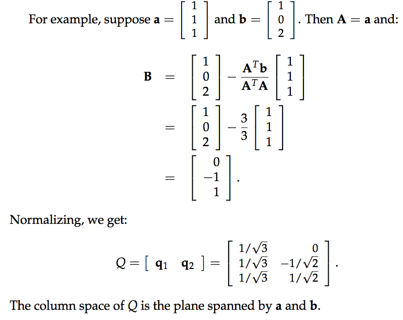
When we studied elimination, we wrote the process in terms of matrices and found A = LU. A similar equation A = QR relates our starting matrix A to the result Q of the Gram-Schmidt process. Where L was lower triangular, R is upper triangular.

If R is upper triangular, then it should be true that $a_1^Tq_2 = 0$. This must be true
because we chose $q_1$ to be a unit vector in the direction of $a_1$. All the later $q_i$
were chosen to be perpendicular to the earlier ones. Notice that $R = Q^TA$. This makes sense; $Q^TQ = I$.

Determinants and Eigenvalues

Properties of Determinants

The determinant is a number associated with any square matrix; we’ll write it as det A or |A|. The determinant encodes a lot of information about the matrix; the matrix is invertible exactly when the determinant is non-zero. We know that $\left|\begin{array}{ll}{a} & {b} \\ {c} & {d}\end{array}\right|=a d-b c$; but the following properties will give us a formula for the determinant of square matrices of all size.

1. $\text{det} I=1$

2. If you exchange two rows of a matrix, you reverse the sign of its determinant from positive to negative or from negative to positive.

3. (A) If we multiply one row of a matrix by $t$, the determinant is multiplied by $t$: $\left|\begin{array}{ll}{ta} & {tb} \\ {c} & {d}\end{array}\right|=t\left|\begin{array}{ll}{a} & {b} \\ {c} & {d}\end{array}\right|$.

   (B) The determinant behaves like a linear function on the rows of the matrix:

   $$\left|\begin{array}{ll}{a+a'} & {b+b'} \\ {c} & {d}\end{array}\right|=\left|\begin{array}{ll}{a} & {b} \\ {c} & {d}\end{array}\right|+\left|\begin{array}{ll}{a'} & {b'} \\ {c} & {d}\end{array}\right|$$

4. If two rows of a matrix are equal, its determinant is zero.

   This is because of property 2, the exchange rule. On the one hand, exchanging the two identical rows does not change the determinant. On the other hand, exchanging the two rows changes the sign of the determinant. Therefore the determinant must be 0.

5. If $i \ne j$, subtracting $t$ times row $i$ from row $j$ doesn’t change the determinant.

   $$\begin{aligned}\left|\begin{array}{cc}{a} & {b} \\ {c-t a} & {d-t b}\end{array}\right| &=\left|\begin{array}{cc}{a} & {b} \\ {c} & {d}\end{array}\right|-\left|\begin{array}{cc}{a} & {b} \\ {t a} & {t b}\end{array}\right| & \text { property } 3(b) \\ &=\left|\begin{array}{cc}{a} & {b} \\ {c} & {d}\end{array}\right|-t\left|\begin{array}{cc}{a} & {b} \\ {a} & {b}\end{array}\right| \quad \text { property } 3(a) \\ &=\left|\begin{array}{cc}{a} & {b} \\ {c} & {d}\end{array}\right| & \text { property } 4 \end{aligned}$$

6. If $A$ has a row that is all zeros, then $\text{det} A=0$. We get this from property 3(A) by letting $t=0$.

7. The determinant of a triangular matrix is the product of the diagonal
   entries (pivots) $d_1,d_2,…,d_n$.

   Property 5 tells us that the determinant of the triangular matrix won’t change if we use elimination to convert it to a diagonal matrix with the entries di on its diagonal. Then property 3 (a) tells us that the determinant of this diagonal matrix is the product $d_1d_2 · · · d_n$ times the determinant of the identity matrix. Property 1 completes the argument.

   Note that we cannot use elimination to get a diagonal matrix if one of the $d_i$ is zero. In that case elimination will give us a row of zeros and property 6 gives us the conclusion we want.

8. $\text{det} A=0$ exactly when $A$ is singular.

   If A is singular, then we can use elimination to get a row of zeros, and property 6 tells us that the determinant is zero. If A is not singular, then elimination produces a full set of pivots $d_1, d_2, …, d_n$ and the determinant is $d_1d_2 · · · d_n \ne 0$ (with minus signs from row exchanges).

9. $\text{det}AB=(\text{det}A)(\text{det}B)$

   This is very useful. Although the determinant of a sum does not equal the sum of the determinants, it is true that the determinant of a product equals the product of the determinants.

   For example:

   $$\text{det}A^{-1}=\frac{1}{\text{det}A}$$

   because $A^{-1}A=1.$ (Note that if $A$ is singular then $A^{-1}$ does not exist and $\text{det}A^{-1}$ is undefined.) Also, $\text{det}A^2=(\text{det}A)^2$ and $\text{det}2A=2^n\text{det}A$ (applying property 3 to each row of the matrix). This reminds us of volume – if we double the length, width and height of a three dimensional box, we increase its volume by a multiple of $2^3=8$.

10. $\text{det}A^T=\text{det}A$.

    $$\left|\begin{array}{ll}{a} & {b} \\ {c} & {d}\end{array}\right|=\left|\begin{array}{cc}{a} & {c} \\ {b} & {d}\end{array}\right|=a d-b c$$

    To see why $|A^T|=|A|$, use elimination to write $A=LU$. The statement becomes $|U^TL^T|=|LU|$. Rule 9 then tells us $|U^T||L^T|=|L||U|$. Matrix $L$ is a lower triangular matrix with 1’s on the diagonal, so rule 5 tells us that $|L|=|L^t|=1$. Because $U$ is upper triangular, rule 5 tells us that $|U|=|U^T|$. Therefore $|U^T||L^T|=|L||U|$ and $|A^T|=|A|$.

Determinant Formulas

Firstly, we try to find a formula for the $2 \times 2$ matrix:

$$\begin{aligned}\left|\begin{array}{cc}{a} & {b} \\ {c} & {d}\end{array}\right| &=\left|\begin{array}{cc}{a} & {0} \\ {c} & {d}\end{array}\right|+\left|\begin{array}{cc}{0} & {b} \\ {c} & {d}\end{array}\right| \\ &=\left|\begin{array}{cc}{a} & {0} \\ {c} & {0}\end{array}\right|+\left|\begin{array}{cc}{a} & {0} \\ {0} & {0}\end{array}\right|+\left|\begin{array}{cc}{0} & {b} \\ {c} & {0}\end{array}\right|+\left|\begin{array}{cc}{0} & {b} \\ {c} & {0}\end{array}\right|+\left|\begin{array}{cc}{0} & {b} \\ {0} & {d}\end{array}\right| \\ &=0+a d+(-c b)+0 \\ &=a d-b c \end{aligned}$$

By applying property 3 (The determinant is linear in each row separately) to separate the individual entries of each row we could get a formula for any other square matrix. However, for a 3 by 3 matrix we’ll have to add the determinants of twenty seven different matrices! Many of those determinants are zero. The non-zero pieces are:

$$\left|\begin{array}{ccc}{a_{11}} & {a_{12}} & {a_{13}} \\ {a_{21}} & {a_{22}} & {a_{23}} \\ {a_{31}} & {a_{32}} & {a_{33}}\end{array}\right|=\left|\begin{array}{ccc}{a_{11}} & {0} & {0} \\ {0} & {a_{22}} & {0} \\ {0} & {0} & {a_{33}}\end{array}\right|+\left|\begin{array}{ccc}{a_{11}} & {0} & {0} \\ {0} & {0} & {a_{23}} \\ {0} & {a_{32}} & {0}\end{array}\right|+\left|\begin{array}{ccc}{0} & {a_{12}} & {0} \\ {a_{21}} & {0} & {0} \\ {0} & {0} & {a_{33}}\end{array}\right| \\ +\left|\begin{array}{ccc}{0} & {a_{12}} & {0} \\ {0} & {0} & {a_{23}} \\ {a_{31}} & {0} & {0}\end{array}\right|+\left|\begin{array}{ccc}{0} & {0} & {a_{13}} \\ {a_{21}} & {0} & {0} \\ {0} & {a_{32}} & {0}\end{array}\right|+\left|\begin{array}{ccc}{0} & {0} & {a_{13}} \\ {0} & {a_{22}} & {0} \\ {a_{31}} & {0} & {0}\end{array}\right|\\ =a_{11}a_{22}a_{33}-a_{11}a_{23}a_{33}-a_{12}a_{21}a_{33}+a_{12}a_{23}a_{31}+a_{13}a_{21}a_{32}-a_{13}a_{22}a_{31}$$

Each of the non-zero pieces has one entry from each row in each column, as in a permutation matrix. Since the determinant of a permutation matrix is either 1 or -1, we can again use property 3 to find the determinants of each of these summands and obtain our formula.

The number of parts with non-zero determinants was 2 in the 2 by 2 case, 6 in the 3 by 3 case, and will be $24=4!$ in the 4 by 4 case. This is because there are n ways to choose an element from the first row, after which there are only n − 1 ways to choose an element from the second row that avoids a zero determinant. Then there are n − 2 choices from the third
row, n − 3 from the fourth, and so on. The big formula for computing the determinant of any square matrix is:

$$\operatorname{det} A=\sum_{n ! \text { terms }} \pm a_{1 \alpha} a_{2 \beta} a_{3 \gamma} \ldots a_{n \omega}$$

where $(\alpha, \beta,\gamma, …, \varpi )$ is some permutation of $(1,2,3,..,n)$.

Cofactor formula

The cofactor formula rewrites the big formula for the determinant of an n by n matrix in terms of the determinants of smaller matrices. In the $3 \times 3$ case, the formula looks like:

$$\begin{aligned} \operatorname{det} A &=a_{11}\left(a_{22} a_{33}-a_{23} a_{32}\right)+a_{12}\left(-a_{21} a_{33}+a_{23} a_{31}\right)+a_{13}\left(a_{21} a_{32}-a_{22} a_{31}\right) \\ &=\left|\begin{array}{ccc}{a_{11}} & {0} & {0} \\ {0} & {a_{22}} & {a_{23}} \\ {0} & {a_{32}} & {a_{33}}\end{array}\right|+\left|\begin{array}{ccc}{0} & {a_{12}} & {0} \\ {a_{21}} & {0} & {a_{23}} \\ {a_{31}} & {0} & {a_{33}}\end{array}\right|+\left|\begin{array}{ccc}{0} & {0} & {a_{13}} \\ {a_{21}} & {a_{22}} & {0} \\ {a_{31}} & {a_{32}} & {0}\end{array}\right| \end{aligned}$$

Each element is multiplied by the cofactors in the parentheses following it. Note that each cofactor is (plus or minus) the determinant of a two by two matrix. Thatdeterminant is made up of products of elements in the rows and columns NOT containing $a_{1j}$.

In general, the cofactor $C_{ij}$ of $a_{ij}$ can be found by looking at all the terms in the big formula that contain $a_{ij}$. $C_{ij}$ equals $(-1)^{i+j}$ times the determinant of the $n-1$ by $n-1$ square matrix obtained by removing row $i$ and column $j$. ($C_{ij}$ is positive if $i+j$ is even.)

For $n \times n$ matrices, the cofactor formula is:

$$\text{det}A=a_{11}C_{11}+a_{12}C_{12}+...+a_{1n}C_{1n}$$

Inverse matrix formula

We know:

$$\left[\begin{array}{ll}{a} & {b} \\ {c} & {d}\end{array}\right]^{-1}=\frac{1}{a d-b c}\left[\begin{array}{rr}{d} & {-b} \\ {-c} & {a}\end{array}\right]$$

In fact: $A^{-1}=\frac{1}{\text{det}A}C^T$, where $C$ is the matrix of cofactors.

To more formally verify the formula, we’ll check that $AC^T=\text{(detA)}I$.

$$A C^{T}=\left[\begin{array}{ccc}{a_{11}} & {\cdots} & {a_{1 n}} \\ {\vdots} & {\ddots} & {\vdots} \\ {a_{n 1}} & {\cdots} & {a_{n n}}\end{array}\right]\left[\begin{array}{ccc}{C_{11}} & {\cdots} & {C_{n 1}} \\ {\vdots} & {\ddots} & {\vdots} \\ {C_{1 n}} & {\cdots} & {C_{n n}}\end{array}\right]$$

The entry in the first row and first column of the product matrix is:

$$\sum_{j=1}^na_{1j}C_{j1}=\text{det}A$$

(This is just the cofactor formula for the determinant.) This happens for every entry on the diagonal of $AC^T$. To finish proving that $AC^T=(\text{det}A)I$, we just need to check that the offdiagonal entries of $AC^T$ are zero. In the two by two case, multiplying the entries in row 1 of $A$ by the entries in column 2 of $C^T$ gives $a(-b)+b(a)=0$. This is the determinant of $A_{S}=\left[\begin{array}{ll}{a} & {b} \\ {a} & {b}\end{array}\right]$. In higher dimensions, the product of the first row of $A$ and the last column of $C^T$ equals the the determinant of a matrix whose first and last rows are identical. This happens with all the off diagonal matrices, which confirms that $A^{-1}=\frac{1}{\text{det}A}C^T$.

Cramer’s rule for $x=A^{-1}b$

We know that if $Ax=b$ and $A$ is nonsingular, then $x=A^{-1}b$. Applying the formula $A^{-1}=\frac{C^T}{\text{det}A}$ gives us:

$$x=\frac{C^Tb}{\text{det}A}$$

Cramer’s rule gives us another way of looking at this equation. To derive this rule we break x down into its components. Because the i’th component of $C^Tb$ is a sum of cofactors times some number, it is the determinant of some matrix $B_j$.

$$x=\frac{\text{det}B_J}{\text{det}A}$$

where $B_j$ is the matrix created by starting with $A$ and then replacing column $j$ with $b$, so

$$\begin{aligned} B_{1} &=\left[\begin{array}{c}{\text { last } \mathrm{n}-1} \\ {\mathbf{b}} & {\text { columns }} \\ {\text { of } A}\end{array}\right] \\ B_{n} &=\left[\begin{array}{cc}{\text { first } \mathrm{n}-1} \\ {\text { columns }} & {\mathbf{b}} \\ {\text { of } A} & {}\end{array}\right] \end{aligned}$$

Computing inverses using Cramer’s rule is usually less efficient than using elimination.

$|\text{det}A|=$ volume of box

Claim: | det A| is the volume of the box (parallelepiped) whose edges are the column vectors of A. (We could equally well use the row vectors, forming a different box with the same volume.)

If A = I, then the box is a unit cube and its volume is 1. Because this agrees with our claim, we can conclude that the volume obeys determinant property 1.

If A = Q is an orthogonal matrix then the box is a unit cube in a different orientation with volume 1 = det Q . (Because Q is an orthogonal matrix, $Q^TQ=I$ and so det Q = ±1.)

Swapping two columns of A does not change the volume of the box (remembering that det A = det AT) or the absolute value of the determinant (property 2). If we show that the volume of the box also obeys property 3 we’ll have proven | det A| equals the volume of the box.

If we double the length of one column of A, we double the volume of the box formed by its columns. Volume satisfies property 3(a). Property 3(b) says that the determinant is linear in the rows of the matrix:

$$\left|\begin{array}{cc}{a+a^{\prime}} & {b+b^{\prime}} \\ {c} & {d}\end{array}\right|=\left|\begin{array}{cc}{a} & {b} \\ {c} & {d}\end{array}\right|+\left|\begin{array}{cc}{a^{\prime}} & {b^{\prime}} \\ {c} & {d}\end{array}\right|$$

Although it’s not needed for our proof, we can also see that determinants obey property 4. If two edges of a box are equal, the box flattens out and has no volume.

Important note: If you know the coordinates for the corners of a box, then computing the volume of the box is as easy as calculating a determinant. In particular, the area of a parallelogram with edges $\begin{bmatrix}a\\b\end{bmatrix}$ and $\begin{bmatrix}c\\d\end{bmatrix}$is $ad-bc$. The area of a triangle with edges $\begin{bmatrix}a\\b\end{bmatrix}$ and $\begin{bmatrix}c\\d\end{bmatrix}$is $\frac{1}{2}(ad-bc)$.

Eigenvalues and eigenvectors

Definition

A matrix $A$ acts on vectors $x$ like a function does, with input $x$ and output $Ax$. Eigenvectors are vectors for which $Ax$ is parallel to $x$. In other words:

$$Ax=\lambda x$$

In this equation, $x$ is an eigenvector of $A$ and $\lambda $ is an eigenvalue of $A$.

Eignevalue 0

If the eigenvalue $\lambda $ equals 0 then $Ax = 0x = 0$. Vectors with eigenvalue 0 make
up the nullspace of $A$; if A is singular, then $\lambda = 0$ is an eigenvalue of A.

Example

Suppose P is the matrix of a projection onto a plane. For any x in the plane Px = x, so x is an eigenvector with eigenvalue 1. A vector x perpendicular to the plane has Px = 0, so this is an eigenvector with eigenvalue $\lambda = 0$. The eigenvectors of P span the whole space (but this is not true for every matrix).

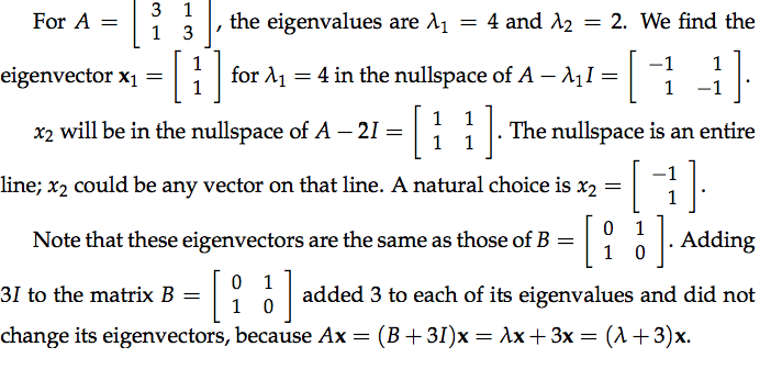
The matrix $B=\begin{bmatrix}0 \ 1 \\ 1 \ 0 \end{bmatrix}$ has an eigenvector $x=\begin{bmatrix} 1 \\ 1 \end{bmatrix}$ with eigenvalue 1 and another eigenvector $x=\begin{bmatrix} 1 \\ -1 \end{bmatrix}$ with eigenvalue -1. These eigenvectors span the space. They are perpendicular because $B=B^T$ (as we will prove).

$\text{det}(A-\lambda I)=0$

An n by n matrix will have n eigenvalues, and their sum will be the sum of the diagonal entries of the matrix: $a_{11}+a_{22}+…+a_{nn}$. This sum is the trace of the matrix. For a two by two matrix, if we know one eigenvalue we can use this fact to find the second.

In order to solve $Ax=\lambda x$ for the eigenvalues and eigenvectors of $A$, we need to be clever to solve this problem:

$$Ax=\lambda x\\ (A-\lambda I)x=0$$

In order for $\lambda $ to be an eigenvector, $A-\lambda I$ must be singular. In other words, $\text{det}(A-\lambda I)=0$. Let $A=\begin{bmatrix}3 \ 1 \\ 1 \ 3 \end{bmatrix}$, then:

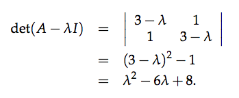
Note that the coefficient 6 is the trace (sum of diagonal entries) and 8 is the determinant of A. In general, the eigenvalues of a two by two matrix are the solutions to:

$$\lambda ^2-\text{trace}(A) \cdot \lambda + \text{det} A=0$$

Just as the trace is the sum of the eigenvalues of a matrix, the product of the eigenvalues of any matrix equals its determinant.

A caution

Similarly, if $Ax=\lambda x$ and $Bx=\alpha x$, $(A+B)x=(\lambda + \alpha)x$. It would be nice if the eigenvalues of a matrix sum were always the sums of the eigenvelues, but this is only true if A and B have the same eigenvectors. The eigenvalues of the product $AB$ are not usually equal to the products $\lambda (A) \lambda (B)$, either.

Complex eigenvalues

The matrix $Q=\begin{bmatrix}0 \ -1 \\ 1 \ 0 \end{bmatrix}$ rotates every vector in the plane by $90^o$. It has trace $0=\lambda_1 +\lambda_2$ and determinant $0=\lambda_1 \cdot \lambda_2$. Its only real eigenvector is the zero vector; any other vector’s direction changes when it is multiplied by $Q$. How will this affect our eigenvalue calculation?

$$\begin{aligned} \operatorname{det}(A-\lambda I) &=\left|\begin{array}{cc}{-\lambda} & {-1} \\ {1} & {-\lambda}\end{array}\right| \\ &=\lambda^{2}+1 \end{aligned}$$

$\text{det}(A-\lambda I)=0$ has solutions $\lambda_1=i$ and $\lambda_2=-i$. If a matrix has a complex eigenvalue $a+bi$ then the complex conjugate $a-bi$ is also en eigenvalue of that matrix.

Symmetric matrices have real eigenvalues. For antisymmetric matrices like $Q$, for which $A^T=-A$, all eigenvalues are imaginary $(\lambda =bi)$.

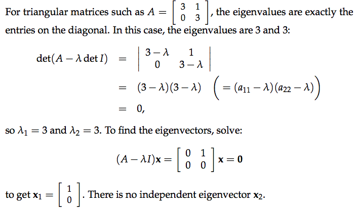
Triangular matrices and repeated eigenvalues

Diagonalization and powers of $A$

Diagonalizing a matrix

If $A$ has $n$ linearly independent eigenvectors, we can put those vectors in the columns of a matrix $S$. Then,

$$\begin{aligned} A S &=A\left[\begin{array}{llll}{\mathbf{x}_{1}} & {\mathbf{x}_{2}} & {\cdots} & {\mathbf{x}_{n}}\end{array}\right] \\ &=\left[\begin{array}{llll}{\mathbf{\lambda}_{1} \mathbf{x}_{1}} & {\lambda_{2} \mathbf{x}_{2}} & {\cdots} & {\lambda_{n} \mathbf{x}_{n}}\end{array}\right] \\ &=\left[\begin{array}{cccc}{\lambda_{1} \mathbf{x}_{1}} & {0} & {\cdots} & {0} \\ {0} & {\lambda_{2}} & {} & {0} \\ {\vdots} & {} & {\ddots} & {\vdots} \\ {0} & {\cdots} & {0} & {\lambda_{n}}\end{array}\right]=S \Lambda \end{aligned}$$

Note that $\Lambda$ is a diagonal matrix whose non-zero entries are the eigenvalues of $A$. Because the columns of $S$ are indepedent, $S^{-1}$ exists and we can multiply both sides of $AS=S\Lambda$ by $S^{-1}$:

$$S^{-1}AS=\Lambda \\ A=S\Lambda S^{-1}$$

Power of $A$

If $Ax=\lambda x$, then $A^2 x = A\lambda x = \lambda Ax = \lambda ^2 x$.

The eigenvalues of $A^2$ are the squares of the eigenvalues of $A$. The eigenvectors of $A^2$ are the same as the eigenvectors of $A$. If we write $A=S\Lambda S^{-1}$ then:

$$A^2=S\Lambda S^{-1}S\Lambda S^{-1}=S\Lambda ^2 S^{-1}$$

Similarly, $A^k=S\Lambda^k S^{-1}$ tells us that raising the eigenvalues of $A$ to the $k$th power gives us the eigenvalues of $A^k$, and that the eigenvectors of $A^k$ are the same as those of $A$.

A is guaranteed to have n independent eigenvectors (and be diagonalizable) if all its eigenvalues are different. Most matrices do have distinct eigenvalues.

Repeated eigenvalues

If A has repeated eigenvalues, it may or may not have n independent eigenvectors. For example, the eigenvalues of the identity matrix are all 1, but that matrix still has n independent eigenvectors.

If $A$ is the triangular matrix $\begin{bmatrix}2 &1\\ 0&2\end{bmatrix}$, its eigenvalues are 2 and 2. Its eigenvectors are in the nullspace of $A-\lambda I=\begin{bmatrix}0 &1\\ 0&0\end{bmatrix}$ which is spanned by $x=\begin{bmatrix}1\\0 \end{bmatrix}$. This particular A does not have two independent eigenvectors.

Difference equations

Start with a given vector $u_0$. We can create a sequence of vectors in which each new vector is A times the previous vector: $u_{k+1}=Au_k$. $u_{k+1}=Au_k$ is a first order difference equation, and $u_k=A^ku_0$ is a solution to this system. We can get a more satisfying solution if we write $u_0$ as a combination of eigenvectors of $A$:

$$u_0=c_1x_1+c_2x_2+\cdot \cdot \cdot +c_nx_n=Sc$$

Then:

$$Au_0=c_1\lambda_1x_1+c_2\lambda_2x_2+\cdot \cdot \cdot +c_n\lambda_nx_n$$

and:

$$u_k=A^ku_0=c_1\lambda_1^kx_1+c_2\lambda_2^kx_2+\cdot \cdot \cdot +c_n\lambda_n^kx_n=\Lambda^kSc$$

Fibonacci sequence

The Fibonacci sequence is $0,1,1,2,3,5,8,13,\cdot\cdot \cdot$ In general, $F_{k+2}=F_{k+1}+F_{k}$. If we could understand this in terms of matrices, the eigenvalues of the matrices would tell us how fast the numbers in the sequence are increasing.

$u_{k+1}=Au_k$ was a first order system. $F_{k+2}=F_{k+1}+F_k$ is a second order scalar equation, but we can convert it to first order linear system by using a clever trick. If $u_k=\begin{bmatrix}F_{k+1} \\ F_k\end{bmatrix}$, then:

$$F_{k+2}=F_{k+1}+F_k\\ F_{k+1}=F_{k+1}$$

is equivalent to the first order system $u_{k+1}=\begin{bmatrix}1&1\\1&0\end{bmatrix}u_k$.

Because $A=\begin{bmatrix}1&1\\1&0\end{bmatrix}$ is symmetric, its eigenvalues will be real and its eigenvectors will be orthogonal.Because A is a two by two matrix we know its eigenvalues sum to 1 (the trace)
and their product is −1 (the determinant).

$$\begin{equation} |A-\lambda I|=\left|\begin{array}{cc}{1-\lambda} & {1} \\ {1} & {-\lambda}\end{array}\right|=\lambda^{2}-\lambda-1 \end{equation}$$

Setting this to zero we find $\lambda = \frac{1\pm \sqrt{1+4}}{2}$; i.e. $\lambda_1 = \frac{1}{2}(1+\sqrt5)\approx 1.618$ and $\lambda_2 = \frac{1}{2}(1-\sqrt5)\approx -0.618$. The growth rate of the $F_k$ is controlled by $\lambda_1$, the only eigenvalue with absolute value greater than 1. This tells us that for large $k$, $F_k \approx c_1 \frac{1+\sqrt{5}}{2}$ for some constant $c_1$. To find the eigenvectors of $A$:

$$\begin{equation} (A-\lambda I) \mathbf{x}=\left[\begin{array}{cc}{1-\lambda} & {1} \\ {1} & {-\lambda}\end{array}\right] \mathbf{x} \end{equation}$$

equals $0$ when $x=\begin{bmatrix}\lambda \\ 1\end{bmatrix}$, so $x_1=\begin{bmatrix}\lambda_1 \\ 1\end{bmatrix}$ and $x_2=\begin{bmatrix}\lambda_2 \\ 1\end{bmatrix}$.

Finally, $u_0=\begin{bmatrix}F_{1} \\ F_0 \end{bmatrix}=\begin{bmatrix}1 \\ 0\end{bmatrix}=c_1x_1+c_2x_x$ tells us that $c_1=-c_2=\frac{1}{\sqrt{5}}$. Because $\begin{bmatrix}F_{k+1} \\ F_k\end{bmatrix}=u_k=c_1\lambda^k_1x_1+c_2\lambda_2^kx_2$, we get:

$$\begin{equation} F_{k}=\frac{1}{\sqrt{5}}\left(\frac{1+\sqrt{5}}{2}\right)^{k}-\frac{1}{\sqrt{5}}\left(\frac{1-\sqrt{5}}{2}\right)^{k} \end{equation}$$

Using eigenvalues and eigenvectors, we have found a closed form expression for the Fibonacci numbers.

Summary: When a sequence evolves over time according to the rules of a
first order system, the eigenvalues of the matrix of that system determine the
long term behavior of the series. To get an exact formula for the series we find
the eigenvectors of the matrix and then solve for the coefficients $c_1, c_2,…$

$e^{At}$ in differential equations

The system of equations below describes how the values of variables $u_1$ and $u_2$ affect each other over time:

$$\begin{equation} \begin{aligned} \frac{d u_{1}}{d t} &=-u_{1}+2 u_{2} \\ \frac{d u_{2}}{d t} &=u_{1}-2 u_{2} \end{aligned} \end{equation}$$

Just as we applied linear algebra to solve a difference equation, we can use it to solve this differential equation. For example, the initial condition $u_1=1,u_2=0$ can written $u(0)=\begin{bmatrix}1\\0\end{bmatrix}$.

By looking at the eigenvalues of the matrix $A=\begin{bmatrix}-1&2\\1&-2\end{bmatrix}$, we can see that $A$ is singular and its trace is $-3$ we know that its eigenvalues are $\lambda_1=0$ and $\lambda_2=-3$. The solution will turn out to include $e^{-3t}$ and $e^{0t}$. As $t$ increases, $e^{-3t}$ vanishes and $e^{0t}=1$ remains constant. Eigenvalues equal to zero have eigenvectors that are steady state solutions.

$x_1=\begin{bmatrix}2\\1\end{bmatrix}$ is an eigenvector for which $Ax_1=0x_1$. To find an eigenvector corresponding to $\lambda_2=-3$ we solve $(A-\lambda_2I)x_2=0$:

$$\begin{bmatrix}2&2\\1&1\end{bmatrix}x_2=0 \ \text{so} \ x_2=\begin{bmatrix}1\\-1\end{bmatrix}$$

The general solution to this system of differential equations will be:

$$u(t)=c_1e^{\lambda_1t}x_1+c_2e^{\lambda_2t}x_2$$

To find out whether $e^{\lambda_1t}x_1$ really a solution to $\frac{du}{dt}=Au$, plug in $u=e^{\lambda_1t}x_1$:

$$\frac{du}{dt}=\lambda_1e^{\lambda_1t}x_1$$

whcih agrees with:

$$Au=e^{\lambda_1t}Ax_1=\lambda_1e^{\lambda_1t}x_1$$

The two pure terms $e^{\lambda_1t}x_1$ and $e^{\lambda_2t}x_2$ are analogous to the terms ${\lambda_i^k}x_i$ we saw in the solution $c_1\lambda_1^kx_1+c_2\lambda_2^kx_2+\cdot \cdot \cdot +c_n\lambda_n^kx_n$ to the difference equation $u_{k+1}=Au_k$.

Plugging in the values of the eigenvectors, we get:

$$\begin{equation} \mathbf{u}(t)=c_{1} e^{\lambda_{1} t} \mathbf{x}_{1}+c_{2} e^{\lambda_{2} t} \mathbf{x}_{2}=c_{1}\left[\begin{array}{c}{2} \\ {1}\end{array}\right]+c_{2} e^{-3 t}\left[\begin{array}{r}{1} \\ {-1}\end{array}\right] \end{equation}$$

we know $u(0)=\begin{bmatrix}1\\0\end{bmatrix}$, so at $t=0$:

$$\begin{bmatrix}1\\0\end{bmatrix} = c_1\begin{bmatrix}2\\1\end{bmatrix}+c_2\begin{bmatrix}1\\-1\end{bmatrix}$$

$c_1=c_2=\frac{1}{3}$ and $u(t)=\frac{1}{3}\begin{bmatrix}2\\1\end{bmatrix}+\frac{1}{3}e^{-3t}\begin{bmatrix}1\-1\end{bmatrix}$ . This tells us that the system starts with $u_1 = 1$ and $u_2 = 0$ but that as t approaches infinity, $u_1$ decays to 2/3 and $u_2$ increases to 1/3. This might describe stuff moving from $u_1$ to $u_2$. The steady state of this system is $u(\infin)=\begin{bmatrix}2/3\\1/3\end{bmatrix}$

Stability

Not all systems have a steady state. The eigenvalues of A will tell us what sort of solutions to expect:

1. Stability: $u(t) \to 0$ when $R(\lambda) < 0$
2. Steady state: One eigenvalue is 0 and all other eigenvalues have negative real part.
3. Blow up: if $R(\lambda )>0$ for any eigenvalue $\lambda$

If a two by two matrix $A=\begin{bmatrix}a&b\\c&d\end{bmatrix}$ has two eigenvalues with negative real part, its trace $a+d$ is negative. If $A$ has a positive determinant and negative trace then the corresponding solutions must be stable.

Applying $S$

The final step of our solution to the system $\frac{du}{dt}=Au$ was to solve:

$$\begin{equation} \begin{array}{l}{c_{1}\left[\begin{array}{l}{2} \\ {1}\end{array}\right]+c_{2}\left[\begin{array}{r}{1} \\ {-1}\end{array}\right]=\left[\begin{array}{l}{1} \\ {0}\end{array}\right]} \\ {\left[\begin{array}{rr}{2} & {1} \\ {1} & {-1}\end{array}\right]\left[\begin{array}{l}{c_{1}} \\ {c_{2}}\end{array}\right]=\left[\begin{array}{l}{1} \\ {0}\end{array}\right]}\end{array} \end{equation}$$

or $Sc=u(0)$, where $S$ is the eigenvector matrix. The components of c determine the contribution from each pure exponential solution, based on the initial conditions of the system. In the equation $\frac{du}{dt}=Au$, the matrix $A$ couples the pure solutions. We set $u=Sv$, where S is the matrix of eigenvectors of A, to get:

$$S\frac{dv}{dt}=ASv$$

or:

$$\frac{dv}{dt}=S^{-1}ASv=\Lambda v$$

This diagonalizes the system: $\frac{dv_i}{dt}=\lambda_i v_i$. The general solution is then:

$$\begin{equation} \begin{aligned} \mathbf{v}(t) &=e^{\Lambda t} \mathbf{v}(0), \quad \text { and } \\ \mathbf{u}(t) &=S e^{\Lambda t} S^{-1} \mathbf{v}(0)=e^{A t} \mathbf{u}(0) \end{aligned} \end{equation}$$

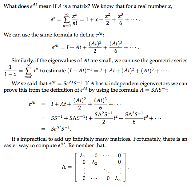
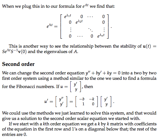
Matrix exponential $e^{At}$

Markov matrices

The eigenvalues of $A$ and the eigenvalues of $A^T$ are the same:

$$(A-\lambda I)^T=A^T-\lambda I$$

so property 10 of determinates tells us that $\text{det}(A-\lambda I)=\text{det}(A^T-\lambda I)$. If $\lambda $ is an eigenvalue of $A$ then:

$$\text{det}(A^T-\lambda I)=0$$

which means $\lambda $ is an eigenvalue of $A^T$.

For a matrix like:

$$A=\begin{bmatrix}0.1&0.01&0.3\\ 0.2&0.99&0.3\\ 0.7&0&0.4\end{bmatrix}$$

in which all entries are non-negative and each column adds to 1 is called a Markov matrix. These requirements come from Markov matrices’ use in probability. Squaring or raising a Markov matrix to a power gives us another Markov matrix.

When dealing with systems of differential equations, eigenvectors with the eigenvalue 0 represented steady states. Here we’re dealing with powers of matrices and get a steady state when $\lambda = 1$ is an eigenvalue.

The constraint that the columns add to 1 guarantees that 1 is an eigenvalue. All other eigenvalues will be less than 1. Remember that (if $A$ has $n$ independent eigenvectors) the solution to $u_k=A^k u_0$ is $u_k = c_1 \lambda_1^k x_1+c_2 \lambda_2^k x_2+\cdot \cdot \cdot +c_n \lambda_n^k x_n$. If $\lambda_1=1$ and all other eigenvalues are less than one, then the system approaches the steady state $c_1x-1$. This is the $x_1$ component of $u_0$.

Why does the fact that the columns sum to 1 guarantee that 1 is an eigenvalue? If 1 is an eigenvalue of A, then:

$$A-1I=\begin{bmatrix}-0.9&0.01&0.3\\ 0.2&-0.01&0.3\\ 0.7&0&-0.6\end{bmatrix}$$

should be singular. Since we’ve subtracted 1 from each diagonal entry, the sum of the entries in each column of A − I is zero. But then the sum of the rows of A-I must be the zero row, and so A-I is singular. The eigenvector $x_1$ is in the nullspace of $A-I$ and has eigenvalue 1. It is not hard to find $x_1=\begin{bmatrix}0.6\\ 0.33\\ 0.7\end{bmatrix}$.

We’re studying the equation $u_{k+1} = Au_k$ where A is a Markov matrix. For example $u_1$ might be the population of (number of people in) Massachusetts and $u_2$ might be the population of California. A might describe what fraction of the population moves from state to state, or the probability of a single personmoving. We can’t have negative numbers of people, so the entries of A will always be positive. We want to account for all the people in our model, so the columns of A add to 1 = 100%. For example:

$$\begin{bmatrix}u_{Cal} \\ u_{Mass} \end{bmatrix}_{t=k+1}=\begin{bmatrix}0.9&0.2 \\ 0.1&0.8 \end{bmatrix}\begin{bmatrix}u_{Cal} \\ u_{Mass} \end{bmatrix}_{t=k}$$

assumes that there’s a 90% chance that a person in California will stay in California and only a 10% chance that she or he will move, while there’s a 20% percent chance that a Massachusetts resident will move to California. If our initial conditions are $\begin{bmatrix}u_{Cal} \\ u_{Mass} \end{bmatrix}_{t=1}=\begin{bmatrix}0 \\ 1000 \end{bmatrix}$, then after one move $u_1=Au_0$ is:

$$\begin{bmatrix}u_{Cal} \\ u_{Mass} \end{bmatrix}_{t=1}=\begin{bmatrix}0.9&0.2 \\ 0.1&0.8 \end{bmatrix}\begin{bmatrix}0\\1000 \end{bmatrix}=\begin{bmatrix}200\\800 \end{bmatrix}$$

For the next few values of $k$, the Massachusetts population will decrease and the California population will increase while the total population remains constant at 1000.

To understand the long term behavior of this system we’ll need the eigen­vectors and eigenvalues of $\begin{bmatrix}0.9&0.2 \\ 0.1&0.8 \end{bmatrix}$. We know that one eigenvalue is $\lambda_1=1$. Becasue the trace 0.9+0.8=1.7 is the sum of the eigenvalues, we see that $\lambda_2=0.7$. Next we calculate the eigenvectors: $x_1=\begin{bmatrix}2 \\1 \end{bmatrix}$ . The eigenvalue 1 corresponds to the steady state solution, and $\lambda_2=0.7 <1$, so the system approaches a limit in which $\frac{2}{3}$ of 1000 people live in Californina and $\frac{1}{3}$ of 1000 people are in Massachusetts. This will be the limit frim any starting vector $u_0$.

To know how the population is distributed after a finite number of steps we look for an eigenvector corresponding to $\lambda_2=0.7$ is $x_2=\begin{bmatrix}1 \-1 \end{bmatrix}$. From what we learned about difference equation we know that:

$$\begin{equation} \mathbf{u}_{k}=c_{1} 1^{k}\left[\begin{array}{l}{2} \\ {1}\end{array}\right]+c_{2}(.7)^{k}\left[\begin{array}{r}{-1} \\ {1}\end{array}\right] \end{equation}$$

when $k=0$ we have:

$$\begin{equation} \mathbf{u}_{0}=\left[\begin{array}{r}{0} \\ {1000}\end{array}\right]=c_{1}\left[\begin{array}{l}{2} \\ {1}\end{array}\right]+c_{2}\left[\begin{array}{r}{-1} \\ {1}\end{array}\right] \end{equation}$$

so $c_1=\frac{1000}{3}$ and $c_2=\frac{2000}{3}$

Fourier series

Expansion with an orthonormal basis

If we have an orthonormal basis $q_1, q_2,…,q_n$ then we can write any vector $v$ as $v+x_1q_1+x_2q_x+\cdot \cdot \cdot +x_nq_n$, where:

$$\begin{equation} \mathbf{q}_{i}^{T} \mathbf{v}=x_{1} \mathbf{q}_{i}^{T} \mathbf{q}_{1}+x_{2} \mathbf{q}_{i}^{T} \mathbf{q}_{2}+\cdots+x_{n} \mathbf{q}_{i}^{T} \mathbf{q}_{n}=x_{i} \end{equation}$$

since $q_i^Tq_j=0$ unless $i=j$, this equation gives $x_i=q_i^Tv$.

In terms of matrices, $\begin{bmatrix}q_1 &\cdot \cdot \cdot & q_n\end{bmatrix}\begin{bmatrix}x_1 \\ \cdot \\ \cdot \\ \cdot \\ q_n\end{bmatrix}=v$, or $Qx=v$. So $x=Q^{-1}v$. Because the $q_i$ form an orthonormal basis, $Q^{-1}=Q^T$ and $x=Q^Tv$. This another way to see that $x_i=q_i^Tv$.

Fourier series

The key idea above was that the basis of vectors $q_i$ was orthonormal. Fourier series are built on this idea. We can describe a function $f(x)$ in terms of trigonometric functions:

$$f(x)=a_0+a_1cosx+b_1sinx+a_2cos2x+b_2sin2x+\cdot \cdot \cdot$$

This Fourier series is an infinite sum and the previous example was finite, but the two are related by the fact that the cosines and sines in the Fourier series are orthogonal. We’re now working in an infinite dimensional vector space. The vectors in this space are functions and the (orthogonal) basis vectors are $1, cosx, sinx, cos2x, sin2x, \cdot \cdot \cdot$

What does “orthogonal” mean in this context? How do we compute a dot product or inner product in this vector space? For vectors in $R^n$ the inner product is $v^Tw=v_1w_1+v_2w_2+ \cdot \cdot \cdot+v_nw_n$. Functions are described by a continuing of values $f(x)$ rather than by a discrete collection of components $v_i$. The best parallel to the vector dot product is:

$$f^Tg=\int_{0}^{2\pi} f(x)g(x)dx$$

We integrate from 0 to 2π because Fourier series are periodic:

$$f(x)=f(x+2\pi)$$

The inner product of two basis vectors is zero, as desired. For example,

$$\begin{equation} \int_{0}^{2 \pi} \sin x \cos x d x=\left.\frac{1}{2}(\sin x)^{2}\right|_{0} ^{2 \pi}=0 \end{equation}$$

How do we find $a_0, a_1$, etc. to find the coordinates or Fourier coefficients of a function in this space? The constant term $a_0$ is the average value of the function. Because we’re working with an orthonormal basis, we can use the inner product to find the coefficients ai.

$$\begin{equation} \begin{aligned} \int_{0}^{2 \pi} f(x) \cos x d x &=\int_{0}^{2 \pi}\left(a_{0}+a_{1} \cos x+b_{1} \sin x+a_{2} \cos 2 x+\cdots\right) \cos x d x \\ &=0+\int_{0}^{2 \pi} a_{1} \cos ^{2} x d x+0+0+\cdots \\ &=a_{1} \pi \end{aligned} \end{equation}$$

we conclude that $a_1=\frac{1}{\pi} \int_0^{2\pi}f(x)cosxdx$. We can use the same technique to find any of the values $a_i$.