All kinds of Machine learning methods.
Maximum Likelihood Estimation
Maximum likelihood estimation is a method that determines values for the parameters of a model. The parameter values are found such that they maximise the likelihood that the data produced by the model were actually observed.
Intuitive explanation
Let’s suppose we have observed 10 data points from some process. For example, each data point could represent the length of time in seconds that it takes a student to answer a specific exam question. These 10 data points are shown in the figure below
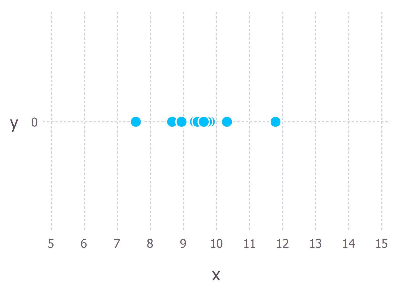
We first have to decide which model we think best describes the process of generating the data. This part is very important. At the very least, we should have a good idea about which model to use. For these data we’ll assume that the data generation process can be adequately described by a Gaussian (normal) distribution. Visual inspection of the figure above suggests that a Gaussian distribution is plausible because most of the 10 points are clustered in the middle with few points scattered to the left and the right.
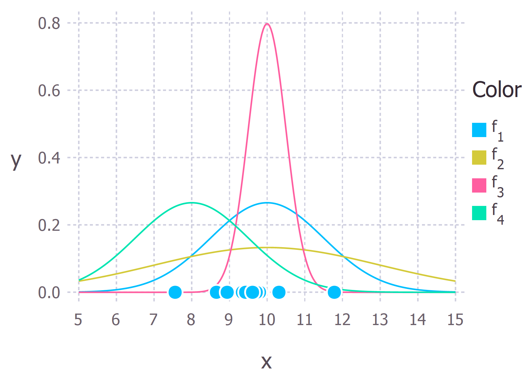
Recall that the Gaussian distribution has 2 parameters. The mean, $\mu$, and the standard deviation, $\sigma$. Different values of these parameters result in different curves (just like with the straight lines above). We want to know which curve was most likely responsible for creating the data points that we observed? (See figure below). Maximum likelihood estimation is a method that will find the values of μ and σ that result in the curve that best fits the data.
Calculating the Maximum Likelihood Estimates
Now that we have an intuitive understanding of what maximum likelihood estimation is we can move on to learning how to calculate the parameter values. The values that we find are called the maximum likelihood estimates (MLE).
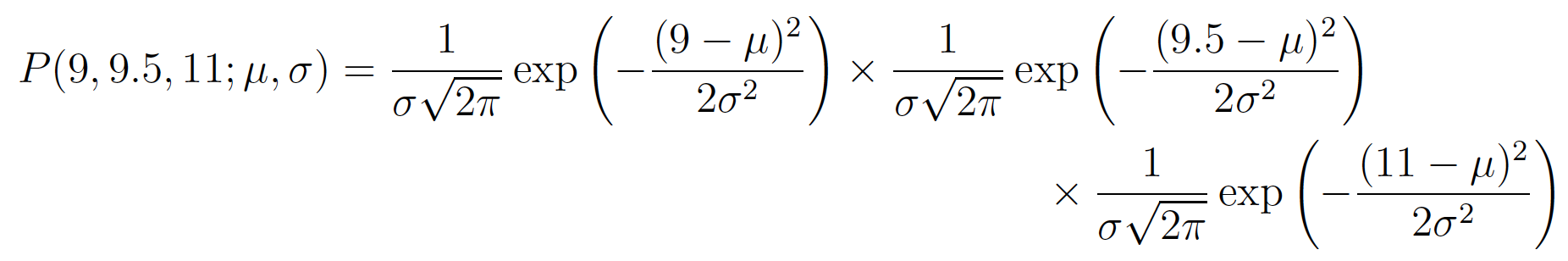
Again we’ll demonstrate this with an example. Suppose we have three data points this time and we assume that they have been generated from a process that is adequately described by a Gaussian distribution. These points are 9, 9.5 and 11. How do we calculate the maximum likelihood estimates of the parameter values of the Gaussian distribution $\mu$ and $\sigma$?
What we want to calculate is the total probability of observing all of the data, i.e. the joint probability distribution of all observed data points. To do this we would need to calculate some conditional probabilities, which can get very difficult. So it is here that we’ll make our first assumption. The assumption is that each data point is generated independently of the others. This assumption makes the maths much easier. If the events (i.e. the process that generates the data) are independent, then the total probability of observing all of data is the product of observing each data point individually (i.e. the product of the marginal probabilities).
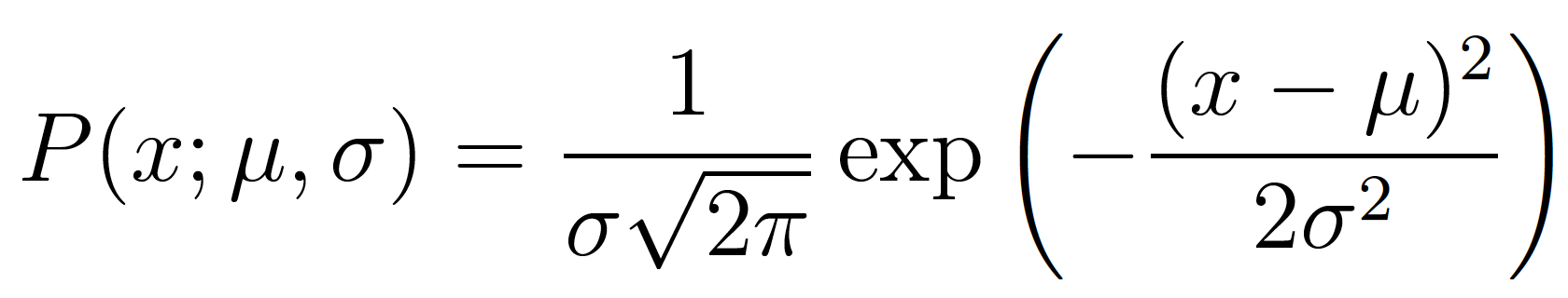
The probability density of observing a single data point $x$, that is generated from a Gaussian distribution is given by:
In our example the total (joint) probability density of observing the three data points is given by:
We just have to figure out the values of $\mu$ and $\sigma$ that results in giving the maximum value of the above expression.
If you’ve covered calculus in your maths classes then you’ll probably be aware that there is a technique that can help us find maxima (and minima) of functions. It’s called differentiation. All we have to do is find the derivative of the function, set the derivative function to zero and then rearrange the equation to make the parameter of interest the subject of the equation.
The log likelihood
The above expression for the total probability is actually quite a pain to differentiate, so it is almost always simplified by taking the natural logarithm of the expression. Taking logs of the original expression gives us:
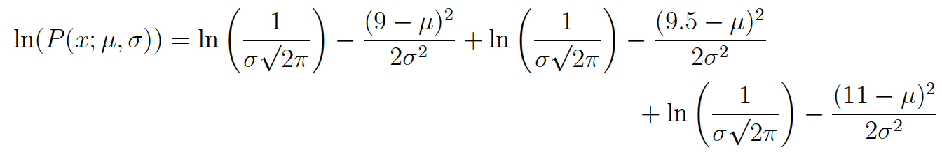
This expression can be simplified again using the laws of logarithms to obtain:

This expression can be differentiated to find the maximum. In this example we’ll find the MLE of the mean, $\mu$. To do this we take the partial derivative of the function with respect to $\mu$, giving

Finally, setting the left hand side of the equation to zero and then rearranging for $\mu$ gives:

Conclusion
Can maximum likelihood estimation always be solved in an exact manner?
No is the short answer. It’s more likely that in a real world scenario the derivative of the log-likelihood function is still analytically intractable (i.e. it’s way too hard/impossible to differentiate the function by hand). Therefore, iterative methods like Expectation-Maximization algorithms are used to find numerical solutions for the parameter estimates. The overall idea is still the same though.
So why maximum likelihood and not maximum probability?
Well this is just statisticians being pedantic (but for good reason). Most people tend to use probability and likelihood interchangeably but statisticians and probability theorists distinguish between the two. The reason for the confusion is best highlighted by looking at the equation.

These expressions are equal! So what does this mean? Let’s first define P(data; $mu$, $\sigma$)? It means “the probability density of observing the data with model parameters $ mu$ and $\sigma$”. It’s worth noting that we can generalise this to any number of parameters and any distribution.
On the other hand L($mu$, $\sigma$; data) means “the likelihood of the parameters $mu$ and $\sigma$ taking certain values given that we’ve observed a bunch of data.”
The equation above says that the probability density of the data given the parameters is equal to the likelihood of the parameters given the data. But despite these two things being equal, the likelihood and the probability density are fundamentally asking different questions — one is asking about the data and the other is asking about the parameter values. This is why the method is called maximum likelihood and not maximum probability.
When is least squares minimisation the same as maximum likelihood estimation?
Least squares minimisation is another common method for estimating parameter values for a model in machine learning. It turns out that when the model is assumed to be Gaussian as in the examples above, the MLE estimates are equivalent to the least squares method. For a more in-depth mathematical derivation check out these slides.
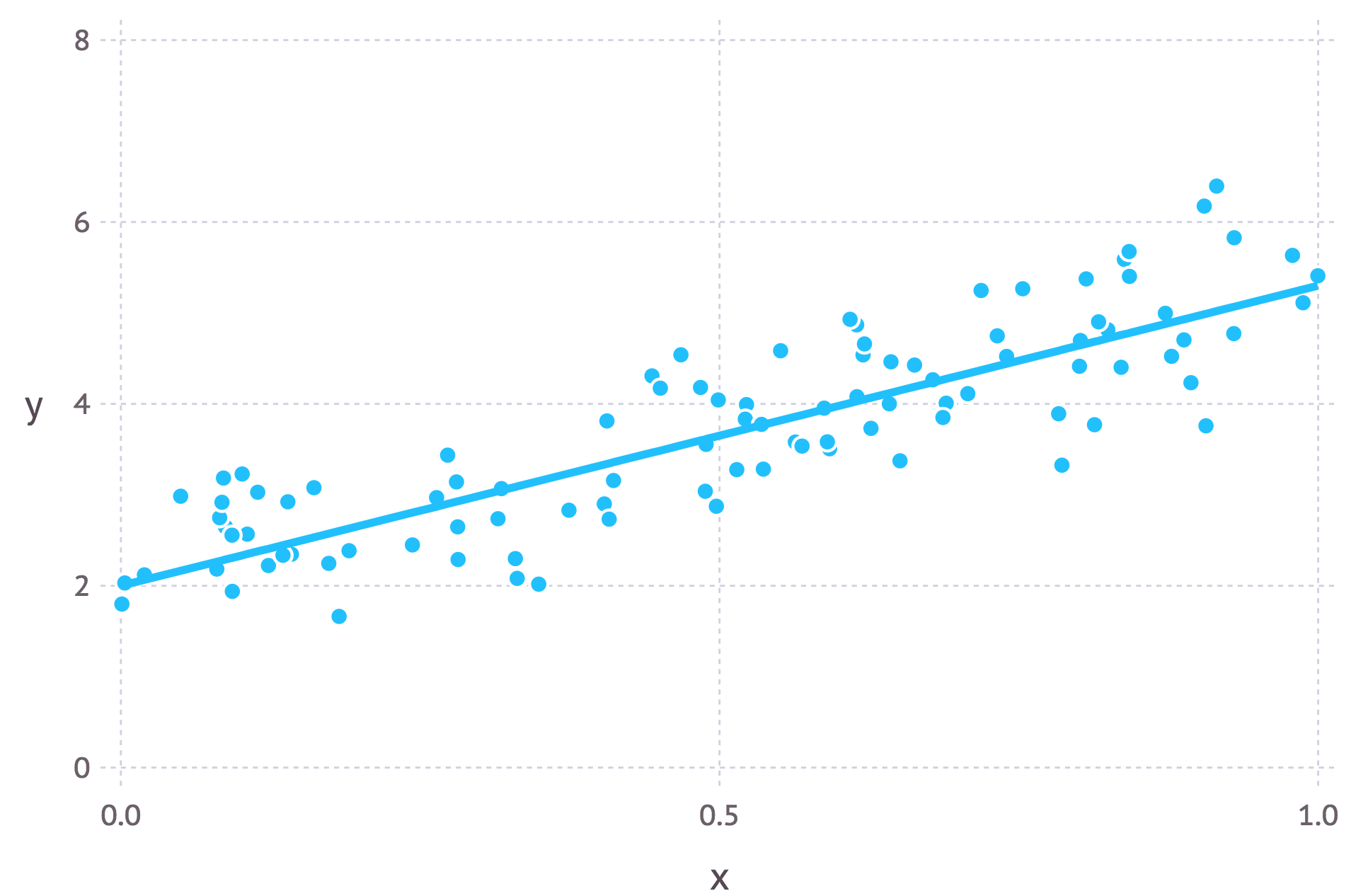
Intuitively we can interpret the connection between the two methods by understanding their objectives. For least squares parameter estimation we want to find the line that minimises the total squared distance between the data points and the regression line (see the figure below). In maximum likelihood estimation we want to maximise the total probability of the data. When a Gaussian distribution is assumed, the maximum probability is found when the data points get closer to the mean value. Since the Gaussian distribution is symmetric, this is equivalent to minimising the distance between the data points and the mean value.
Expectation Maximization
Although Maximum Likelihood Estimation (MLE) and EM can both find “best-fit” parameters, how they find the models are very different. MLE accumulates all of the data first and then uses that data to construct the most likely model. EM takes a guess at the parameters first — accounting for the missing data — then tweaks the model to fit the guesses and the observed data. The basic steps for the algorithm are:
- An initial guess is made for the model’s parameters and a probability distribution is created. This is sometimes called the “E-Step” for the “Expected” distribution.
- Newly observed data is fed into the model.
- The probability distribution from the E-step is tweaked to include the new data. This is sometimes called the “M-step.”
- Steps 2 through 4 are repeated until stability (i.e. a distribution that doesn’t change from the E-step to the M-step) is reached.
Latent Variables
A latent variable model is a type of statistical model that contains two types of variables: observed variables and latent variables. Observed variables are ones that we can measure or record, while latent (sometimes called hidden) variables are ones that we cannot directly observe but rather inferred from the observed variables. One reason why we add latent variables is to model “higher level concepts” in the data, usually these “concepts” are unobserved but easily understood by the modeller. Adding these variables can also simplify our model by reducing the number of parameters we have to estimate.
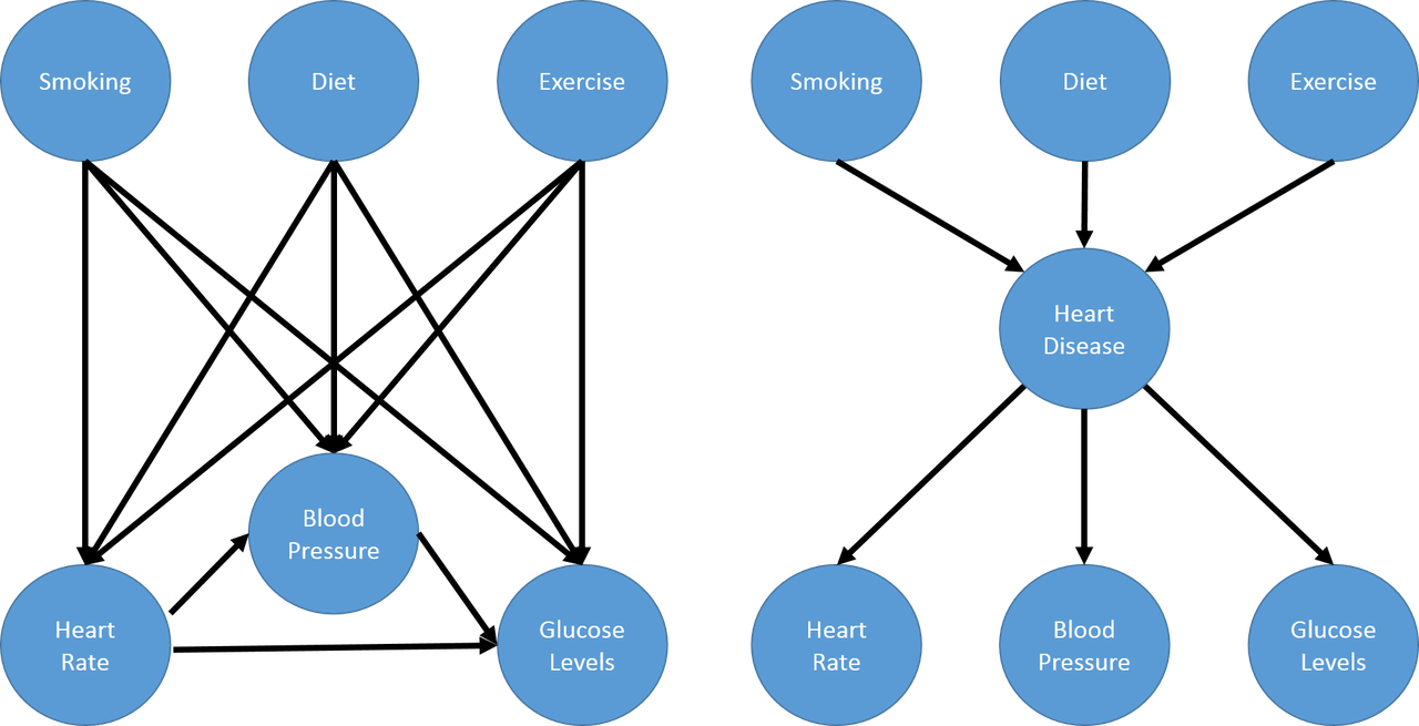
Consider the problem of modelling medical symptoms such as blood pressure, heart rate and glucose levels (observed outcomes) and mediating factors such as smoking, diet and exercise (observed “inputs”). We could model all the possible relationships between the mediating factors and observed outcomes but the number of connections grows very quickly. Instead, we can model this problem as having mediating factors causing a non-observable hidden variable such as heart disease, which in turn causes our medical symptoms. This is shown in the next figure (example taken from Machine Learning: A Probabilistic Perspective).
Gaussian Mixture Models
As an example, suppose we’re trying to understand the prices of houses across the city. The housing price will be heavily dependent on the neighborhood, that is, houses clustered around a neighborhood will be close to the average price of the neighborhood. In this context, it is straight forward to observe the prices at which houses are sold (observed variables) but what is not so clear is how is to observe or estimate the price of a “neighborhood” (the latent variables). A simple model for modelling the neighborhood price is using a Gaussian (or normal) distribution, but which house prices should be used to estimate the average neighborhood price? Should all house prices be used in equal proportion, even those on the edge? What if a house is on the border between two neighborhoods? Can we even define clearly if a house is in one neighborhood or the other? These are all great questions that lead us to a particular type of latent variable model called a Gaussian mixture model.
Following along with this housing price example, let’s represent the price of each house as real-valued random variable $x_i$ and the unobserved neighborhood it belongs to as a discrete valued random variable $z_i$. Further, let’s suppose we have $K$ neighborhoods, therefore $z_i$ can be modelled as a categorical distribution with parameter $\pi=[\pi_1,…,\pi_k]$, and the price distribution of the $k^{th}$ neighborhood as a Gaussian $N(\mu_k,\sigma^{2}_{k})$. The density of $x_i$ is given by:
where $\theta $ represents the parameters of the Gaussians (all the $\mu_k$, $\sigma^2_k$) and the categorical variables $\pi$. $\pi$ represents the prior mixture weights of the neighborhoods.
In the Expectation Step, we assume that the values of all the parameters $(\theta=(\mu_k,\sigma^2_k,\pi))$ are fixed and are set to the ones from the previous iteration of the algorithm. We then just need to compute the responsiblity of each cluster to each point. Re-phasing this problem: Assuming you know the locations of each of the $K$ Gaussians $(\mu_k,\sigma_k)$ , and the prior mixture weights of the Gaussians $(\pi_k)$, what is the probability that a given point $x_i$ is drawn from cluster $k$?
We can write this in terms of probability and use Bayes theorem to find the answer:
The Maximization Step turns things around and assumes the responsibilities (proxies for the latent variables) are fixed, and now the problem is we want to maximize our (expected complete data log) likelihood function across all the $(\theta=(\mu_k,\sigma^2_k,\pi))$ variables.
First up, the distribution of the prior mixture weights $\pi$. Assuming you know all the values of the latent variables; then intuitively, we just need to sum up the contribution to each cluster and normalize:
Next, we need to estimate the Gaussians. Again, since we know the responsibilities of each point to each cluster, we can just use our standard methods for estimating the mean and standard deviation of Gaussians but weighted according to the responsibilities: