This post introduce a new field of machine learning, i.e., meta learning, whose aim is to learn the “learn ability”. For example, we train a model on multiple learning tasks, such as speech recognition, image classification and so on, then when it perform a new task like text classification, it will learn faster and better since it has seen a lot of similar recognition tasks. In a nutshell, meta-learning algorithms produce a base network that is specifically designed for quick adaptation to new tasks using few-shot data.
Introduction
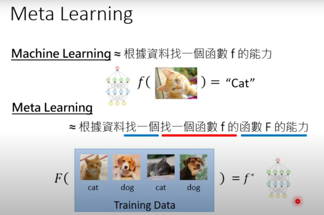
Compare with machine learning, which aims to learn a distribution of data instances from a single task, meta learning tries to generalize over a distribution of tasks. The difference is visualized as follows:
The difference also exists in training dataset. The following figure illustrates the data used in meta learning.
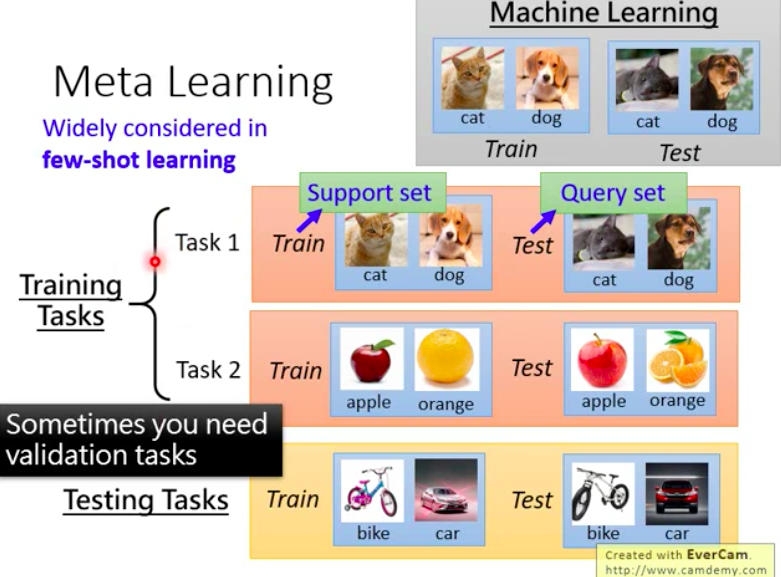
Each training input is a task, whcih includes training images and test images for this particular task. And the test input is a task too, which are unseen during the training. So once we used the training tasks to train the meta model and learnt function is $F$, then the training loss is as following:
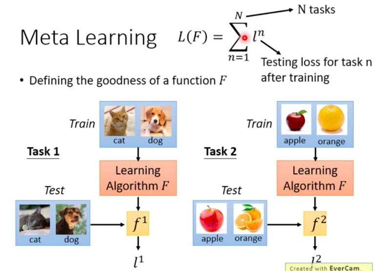
Once the loss function is defined, then our purpose is to find the best function $F^*$
And then this best function is used to test on unseen tasks:
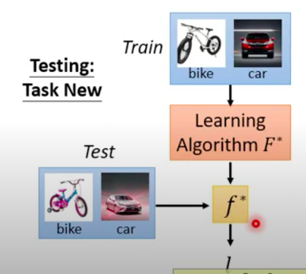
Under this unseen task, we use the train images to find the best discrimination function $f^$ for this task, and then $f^$ is used to classify the unseen test images.
MAML
As one of the most popular meta learning algorithm, model-agnostic meta learning is effective and gain a lot of attention. The following figure illustrates the training process of meta learning.
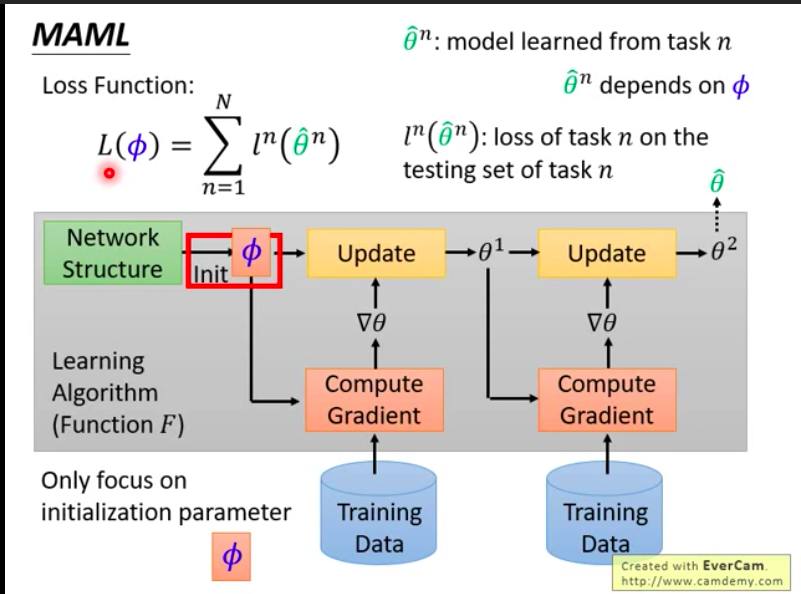
We initialize the model with parameters $\phi$, and our purpose is to learn $\phi$. First we sample a task from training data and compute the gradients on this task, so that we get updated model parameters $\theta ^1$. Therefore the loss for this task is $l(\theta^1)$, which means we use the updated paramters to predict test images of this task and then compute the loss. After that, we sample another task and get updated parameters $\theta ^2$. The loss is $l(\theta^2)$. Accumulating all losses, we can abtain the final loss function:
Compared to transfer learning, which focuses on updating paramters on one new task:
To better undersatnd the difference between meta learning and transfer learning, we can look at the following figures:
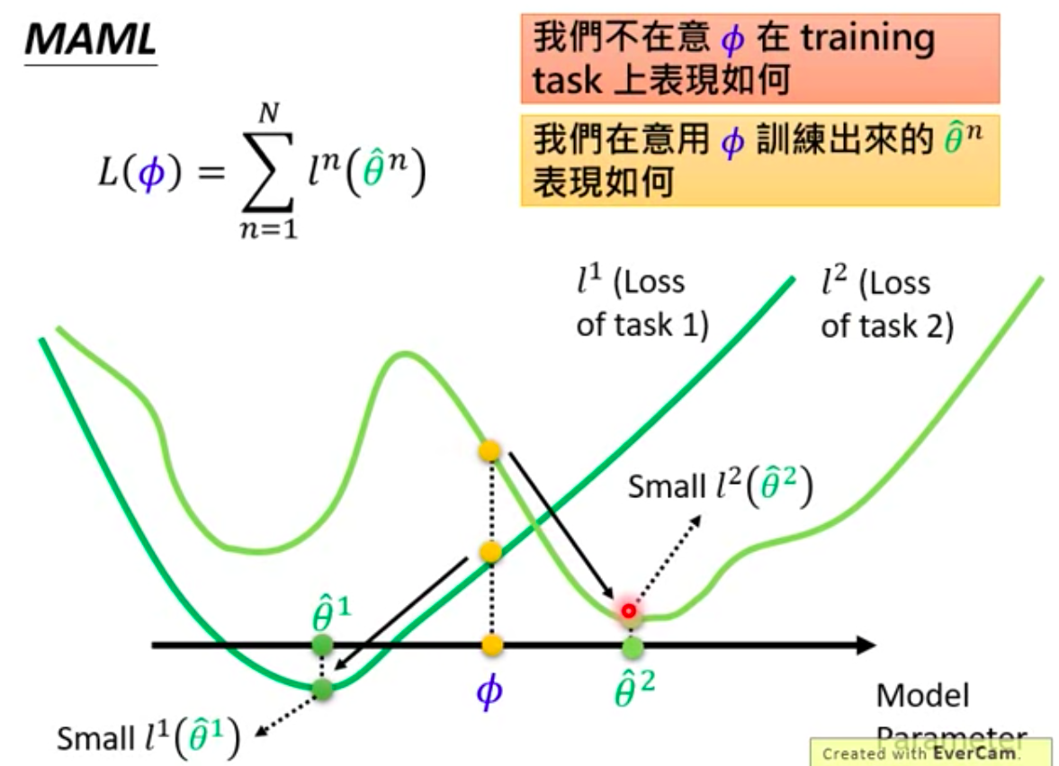
The axis denotes model parameters, while each line denotes the loss function for each task. Say we the current $\phi$ may not be the best parameters for these two tasks because it is not the losses are not least for both lines. However, it may be the best meta learning parametes, because for task one loss line, we can easiler update $\phi$ to the optimal point $\hat \theta^1$. And we can also updtae $\phi$ to the best optimal point $\hat \theta ^2$.
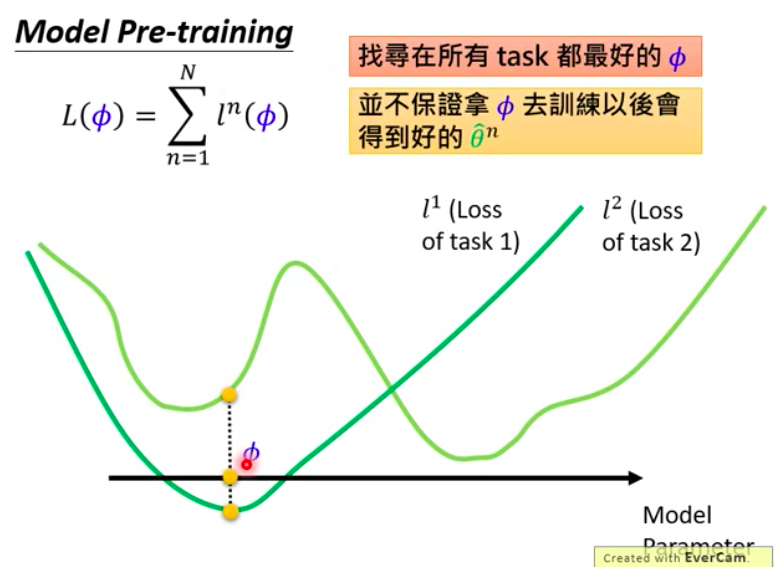
For transfer learning, the best parameters could be on the one of local optimal point of two tasks. Becasue this point performs better on two tasks under this situation.
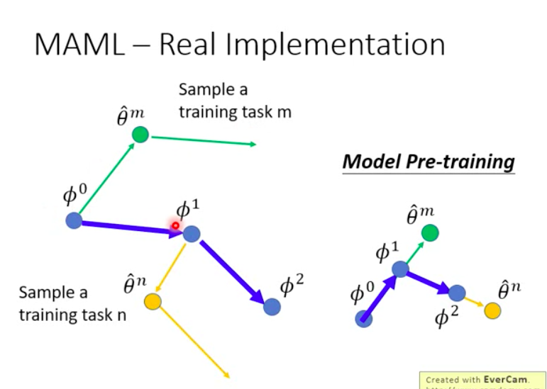
Given the starting parameters $\phi^0$, we update it on training images and get $\hat \theta ^m$, then we test this updated $\hat \theta ^m$ on test images and use the loss to update the original $\phi^0$ to reach the new point $\phi^1$.