线性回归
模型
线性回归模型,顾名思义就是线性模型求解回归问题。
线性模型
【定义】给定具有$d$个属性的数据样本$x=\{x_1,x_2,…,x_d\}$,$x_i$是$x$在第$i$个属性上的取值,线性模型通过对属性的线性组合来进行预测的函数:
向量形式表示为:
其中$w=(w_1;w_2;…;w_d)$,只要确定了$w$和$b$,模型就得以确定。
向量都表示成竖直的一条直线。
回归问题
回归属于监督学习的范畴,用于预测输入变量与输出变量的关系。其本质就是数据拟合,选择一条函数曲线使其很好地拟合已知的数据,同时能够预测未知的数据。
按照输入变量的属性个数,分为一元回归和多元回归;按照输入变量和输出变量之间的映射关系,分为线性回归和非线性回归。
线性回归
线性模型描述的是属性间的组合关系,而回归问题求解的是输入与输出的关系。
即使用一个线性函数去建模输入变量属性间的线性关系,从而发现输入变量与输出变量的关系。给定数据集$D=\{(x_1,y_1),(x_2,y_2),…,(x_m,y_m)\}$,其中$x_i=(x_i1;x_i2;…;x_id)$。
问题描述:线性回归试图学习一个线性模型$f(x_i)=w^Tx_i+b$,使$f(x_i)\approx y_i$。
又称为多元线性回归,或者多变量线性回归。
算法求解
最小二乘法
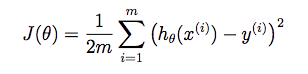
只要确定了权重$w$和偏差$b$的值,那么我们就可以得到模型了,而我们想让预测值$f(x_i)$无限接近真实值$y_i$,所以使用均方误差作为性能度量,即我们试图让均方差最小:
均方误差对应了常用的欧几里得距离,基于均方误差最小化进行模型求解的方法称为“最小二乘法”,实际上,最小二乘法就是试图找到一条直线,使样本到直线的欧氏距离之和最小。
参数估计
Loss函数求导取极值
我们可以对损失函数$Loss$求导,并令导数为零来求得最优参数:
公式推导
偏导
求解b,$\frac{\partial{}E}{\partial{b}}=0$
则$b=\frac{1}{n}\sum_{i=1}^{n}(y_i-wx_i)=\bar{y}-w\bar{x}$
求解w,$\frac{\partial{}E}{\partial{w}}=0$
则$w(\sum_{i=1}^{n}x_{i}^{2}-n\bar{x}^2)=\sum_{i=1}^{n}x_iy_i-n\bar{y}\bar{x}$,故
梯度下降法
损失函数是:
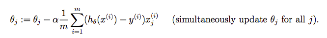
参数更新:
即:
此时,$b=w_0$,$x_0=1$。
正则化的损失函数
此时目标函数为:
$w_0$不需要正则化
此时梯度下降法为:
Data Preprocessing
Feature Scaling
It involves dividing the input values by the range (i.e. the maximum value minus the minimum value) of the input variable, resulting in a new range of just 1.
Mean normalization
This involves subtracting the average value for an input variable from the values for that input variable resulting in a new average value for the input variable of just zero.
By combining the two techniques and adjust the input values as shown in the following formula:
where $\mu_i$ is the average of all the values for feature $(i)$ and $s_i$ is the range of values (max - min), or $s_i$ is the standard deviation.
Convergence Figure
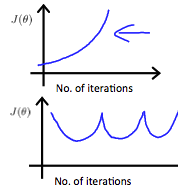
In order to make sure that our algorithm runs correctly, we need to debug gradient descent. Make a plot with number of iterations on the x-axis. Now plot the cost function, $J(\theta)$ over the number of iterations of gradient descent. If $J(\theta)$ ever increases, then you probably need to decrease learning rate $\alpha$.
Summary
If $\alpha$ is too small, it could result in slow convergence.
If $\alpha$ is too large, it may not decrease on every iteration and thus may not converge, like the following pic:
Example
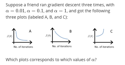
A is $\alpha=0.1$, B is $\alpha=0.01$, A is $\alpha=1$.
In graph C, the cost function is increasing, so the learning rate is set too high. Both graphs A and B converge to an optimum of the cost function, but graph B does so very slowly, so its learning rate is set too low. Graph A lies between the two.
Polynomial Regression
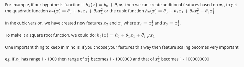
Our hypothesis function need not be linear (a straight line) if that does not fit the data well.
We can change the behavior or curve of our hypothesis function by making it a quadratic, cubic or square root function (or any other form).
例子
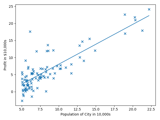
线性回归预测一维数据
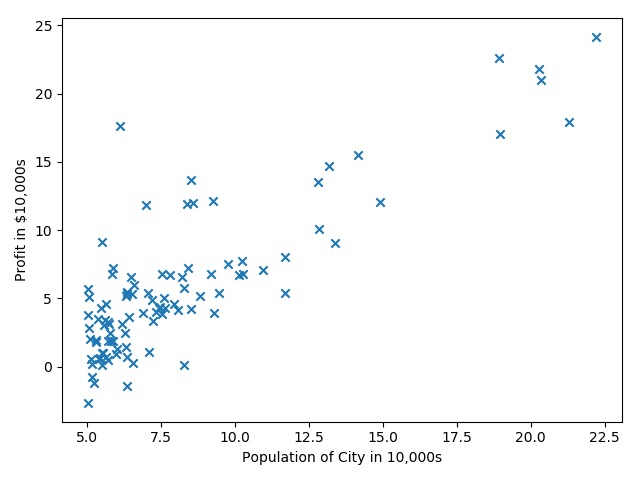
来自Andrew Ng第二周的课程练习,给出城市人口及该市的商店利润,预测如何进行店铺扩展,即选择哪座城市开分店?给定的数据只有一个人口特征及利润目标值。
第一步就是进行数据的可视化。
|
|
第二步:数据处理及参数初始化
我们为数据增加一列全一
|
|
第三步:损失函数
我们使用公式
初次调用,返回值是32.07。
|
|
第四步:梯度下降法
检查梯度下降法是否正确的一个手段:查看损失函数是否在逐步减小。我们使用梯度更新公式:
|
|
需要注意的一个点是:loss = ( y_pred - y )。反过来的话,会出现loss趋于无穷大。这个是对loss函数求导得到的,无论$(h_\theta(x)-y )^2$还是$(y-h_\theta(x) )^2$,都是一样的。
第五步:可视化拟合曲线
|
|
线性回归预测多特征数据
我们使用线性回归预测房价,数据集有两个特征:第一列是房屋面积(单位:$feet^2$),第二列是房间数,最后一列是房价。
特征正则化
发现两个特征数据范围相差特别大,所以需要对数据进行正则化,这样可以加快梯度下降法的收敛。
- 减去均值
- 除以标准差
正则化之后,别忘记加一个全一列。
注意:记得存储mean和std的值,这样我们在预测位置数据的时候,第一步就是使用mean和std对未知数据做同样的处理。
|
|
梯度下降法
先实现损失函数
|
|
再实现梯度下降法,损失函数都是10次方。
|
|