Logistic Regression

Posted on 2018-08-18 | In Machine Learning

用于分类任务的逻辑斯蒂回归。

Python Sth

Posted on 2018-08-09 | In Python

EasyDict

from easydict import EasyDict as edict
mydict = edict({})
mydict.foo = 3
print(mydict.foo) # 3

R & W in TXT

ref

np.loadtxt()用于从文本加载数据。文本文件中的每一行必须含有相同的数据。

1	loadtxt(fname, dtype=<class 'float'>, comments='#', delimiter=None, converters=None, skiprows=0, usecols=None, unpack=False, ndmin=0)

fname：文件名
dtype：数据类型，默认float
comments：注释
delimiter：分隔符，默认是空格
skiprows：跳过前几行，0是第一行，必须int
usecols：要读取哪些列，0是第一列。例如，usecols = （1,4,5）将提取第2，第5和第6列。默认读取所有列。
unpack如果为True，将分列读取。

with open('odom.txt', 'r') as f:
    data = f.readlines()  #txt中所有字符串读入data
 
    for line in data:
        odom = line.split()        #将单个数据分隔开存好
        numbers_float = map(float, odom) #转化为浮点数

TXT追加内容

my_open = open(file_name, 'a')
#打开fie_name路径下的my_infor.txt文件,采用追加模式
#若文件不存在,创建，若存在，追加
my_open.write('xx\n')
my_open.close()

文件操作

文件移动

1 2	import shutil shutil.move(src,des)

Print

pprint

it is used for pretty-print data structures.

Random

np.random.rand()

1	numpy.random.rand(d0,d1,…,dn)

rand函数根据给定维度生成[0,1)之间的数据，包含0，不包含1
dn为每个维度
返回值为指定维度的数组

np.random.randn()

randn函数返回具有标准正态分布的数据。
dn为每个维度
返回值为指定维度的数组

np.random.randint()

numpy.random.randint(low, high, size)

返回开区间 [low, high)范围内的整数值
默认high是None,如果只有low，那范围就是[0,low)。如果有high，范围就是[low,high)
size是输出数组的维度（形状），可以是列表，或者元组

np.random.choice()

numpy.random.choice(a, size)

a可以是一个数或者一个array，如果是一个数则sample范围是【0，a);如果是array，则从中sample
size为sample大小；如果size=(m,n,k)，则采样$mnk$个。

String

数字补0

1 2	n = 123 number = "%05d"%n ### number = 00123

Plt

图片保存去除周边空白ref

1
2
3

plt.figure(figsize=(15,8)) 
p = plt.subplot(111)
plt.savefig('image_name', ,bbox_inches='tight')

bbox_inches =’tight’ 只能用于保存图片，不能用于显示。

Time

1 2	import time start_time = time.time()

Zip

name = [ "Manjeet", "Nikhil", "Shambhavi", "Astha" ] 
roll_no = [ 4, 1, 3, 2 ] 
marks = [ 40, 50, 60, 70 ] 
# using zip() to map values 
mapped = zip(name, roll_no, marks) 
# converting values to print as set 
mapped = set(mapped)

1	The zipped result is : {('Shambhavi', 3, 60), ('Astha', 2, 70), ('Manjeet', 4, 40), ('Nikhil', 1, 50)}

How to unzip?
Unzipping means converting the zipped values back to the individual self as they were. This is done with the help of “*” operator.

name = [ "Manjeet", "Nikhil", "Shambhavi", "Astha" ] 
roll_no = [ 4, 1, 3, 2 ] 
marks = [ 40, 50, 60, 70 ] 
# using zip() to map values 
mapped = zip(name, roll_no, marks) 
# converting values to print as list 
mapped = list(mapped) 
# printing resultant values  
print ("The zipped result is : ",end="") 
print (mapped) 
print("\n") 
# unzipping values 
namz, roll_noz, marksz = zip(*mapped) 
print ("The unzipped result: \n",end="") 
# printing initial lists 
print ("The name list is : ",end="") 
print (namz) 
print ("The roll_no list is : ",end="") 
print (roll_noz) 
print ("The marks list is : ",end="") 
print (marksz)

The zipped result is : [('Manjeet', 4, 40), ('Nikhil', 1, 50), 
('Shambhavi', 3, 60), ('Astha', 2, 70)]
The unzipped result: 
The name list is : ('Manjeet', 'Nikhil', 'Shambhavi', 'Astha')
The roll_no list is : (4, 1, 3, 2)
The marks list is : (40, 50, 60, 70)

Parser

import argparse
    parser = argparse.ArgumentParser(description="Process some parameters.")
    parser.add_argument('--trainFeature', '-tf', type=int, required=True, default=1, help='train feature')
    parser.add_argument('--trainInitial', '-ti', type=int, required=True, default=1,help='train initial')
    parser.add_argument('--learningRate', '-lr', type=float, required=True, default=0.00001,help='learning rate')
    parser.add_argument('--criticNum', '-cn', type=int, required=True, default=5,help='critic number')
    parser.add_argument('--clipRange', '-cr', type=float, required=True,default=0.01, help='clip range')

    args = parser.parse_args()
    opts = {k:v for k,v in args._get_kwagrs()}
    n_critic = args.criticNum
    train_initial = args.trainInitial
    train_feature = args.trainFeature
    lr = args.learningRate
    clip = args.clipRange

    dgan = StageTwo(n_critic,train_initial,train_feature,lr,clip)

1	python xx.py -trainFeature 1 -trainInitial 1 -learningRate 0.001 -criticNum 5 -clipRange 0.01

Matplotlib

5 Quick and Easy Data Visualizations in Python with Code

8 of the best articles on visualizing data

ElementTree

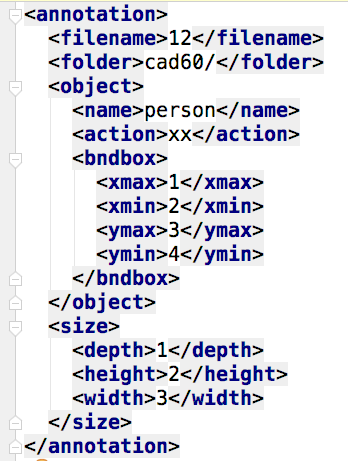
！！！！！所有的输入都必须是字符串！！！！！

def indent(elem, level=0):
  i = "\n" + level*"  "
  if len(elem):
    if not elem.text or not elem.text.strip():
      elem.text = i + "  "
    if not elem.tail or not elem.tail.strip():
      elem.tail = i
    for elem in elem:
      indent(elem, level+1)
    if not elem.tail or not elem.tail.strip():
      elem.tail = i
  else:
    if level and (not elem.tail or not elem.tail.strip()):
      elem.tail = i

def createXML():
    root =ET.Element('annotation')
    filename = ET.Element('filename')
    filename.text = 'xx'
    root.append(filename)

    folder = ET.Element('folder')
    folder.text = 'cad60/'
    root.append(folder)

    object = ET.Element('object')
    root.append(object)

    name = ET.SubElement(object,'name')
    name.text = 'person'
    action = ET.SubElement(object, 'action')
    action.text = '12'
    bndbox = ET.SubElement(object,'bndbox')
    xmax = ET.SubElement(bndbox,'xmax')
    xmax.text = '1'
    xmin = ET.SubElement(bndbox, 'xmin')
    xmin.text = '2'
    ymax = ET.SubElement(bndbox, 'ymax')
    ymax.text = '3'
    ymin = ET.SubElement(bndbox,'ymin')
    ymin.text = '4'

    size = ET.Element('size')
    root.append(size)
    depth = ET.SubElement(size,'depth')
    depth.text = '1'
    height = ET.SubElement(size, 'height')
    height.text = '2'
    width = ET.SubElement(size, 'width')
    width.text = '3'

    indent(root)

    tree = ET.ElementTree(root)
    tree.write('wq.xml','utf-8')

creen Shot 2019-07-27 at 8.41.15 P

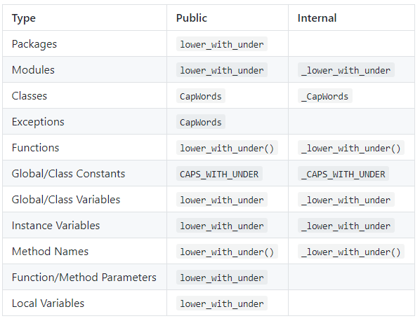
Naming style

ython-namin

Adversarial AutoEncoder

Posted on 2018-08-08 | In Deep Learning

Adversarial Autoencoder

ref1 gocha good one

无监督AAE

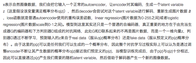
autoencoder中的encoder的输出(潜在码)并不能在某一特定空间均匀分布，而且AE 的 G 只能保证将由 x 生成的 z 还原为 x。如果我们随机生成 1 个 z，经过 AE 的 G 后往往不会得到有效的图像。

所以我们希望encoder的输出可以服从某一分布，这个分布可以是正态分布，均匀分布等，这样就会使encoder的输出均匀分布在给定的先验分布，使decoder学习到一个先验分布到输入数据的映射(本例中就是学习到MNIST手写体数据的分布)，那么此时只需从这个先验分布采样出 z，就能通过 G 得到有效的图像。

假设你正在学习一门课程，如果你的老师并没有提供任何资料，你又会如何学习这门课呢？但是考试怎么办呢，难道要自己瞎答吗？这种情况就是类似我们的encoder的输出并不服从某种特定分布，这样decoder就无法学习到一个从任意数字到图片的映射。

但是如果你有了一个课程指导书，你就可以在考试之前复习这本书，这样就知道了可能的考试内容。类似的，如果我们的encoder输出服从一个已知分布，那么encoder就会将潜在码覆盖整个先验分布。

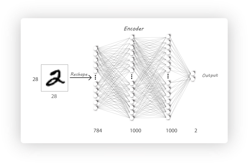
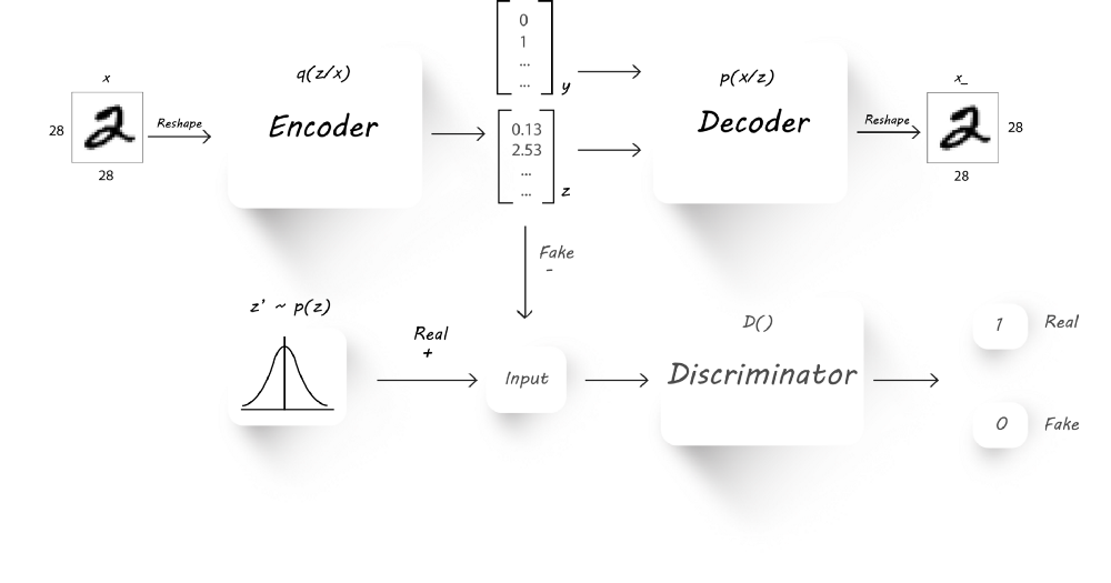
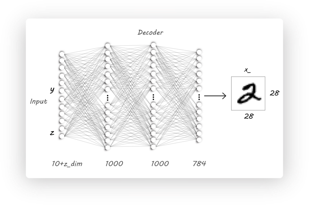
模型

Screen-Shot-2016-10-13-at-11.17.21-AM-690x332

Screen Shot 2018-08-08 at 9.33.36 PM

1_nnf4UUq9Uuf2l19iCYaNfg

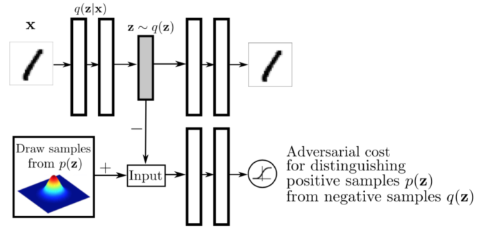
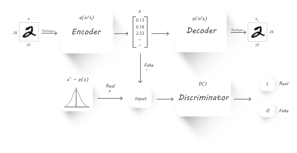
$x$是输入
$q(z|x)$是encoder基于输入$x$的输出
$z$是潜在码，同时也是一个假输入，从$q(z|x)$中采样得到
$z’$是采样自想要的分布，作为真实输入
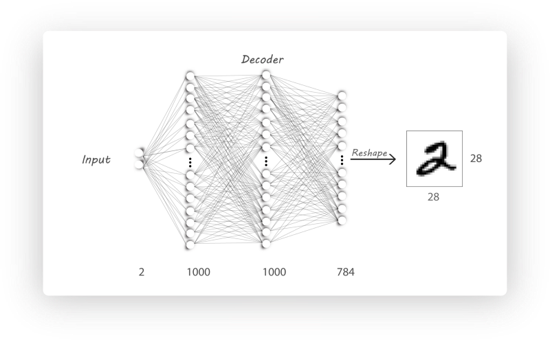
$p(x|z)$是基于$z$的decoder输入
$x_$是重构图像

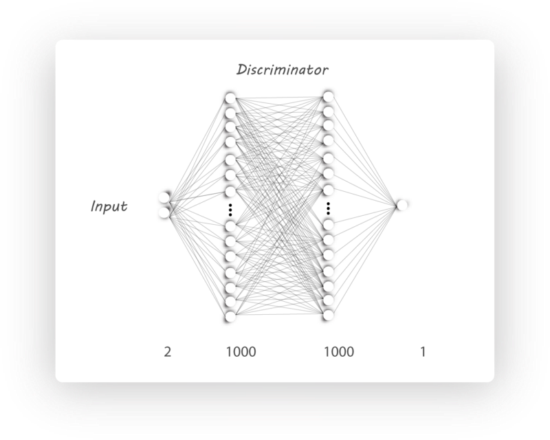
我们的主要目的是迫使encoder的输出逼近一个先验分布（比如正态分布，gamma分布等）。我们将使用encoder$(q(z|x))$作为生成器，而判别器辨别它的输入是来自于一个先验分布$p(z)$，亦或是来自于encoder的输出$z$，decoder仍然进行图片重构的工作。

训练

AAE的训练分成两个部分：重构阶段和正则化阶段。

训练上述模型，分成两个阶段：一个是对辨别器的训练；另一个是对GAN模型的训练。

对于分辨器，其输入就是真假latent code，输出real概率

对于GAN模型，它需要配合分辨器来完成训练。encoder-decoder产生两个输出：一个是latent code，一个是image，但是我们只需要latent code作为分辨器的输入，从而完成GAN模型的训练。

重构阶段

1_DKPl7YOnX-8FJQuHAZop-g

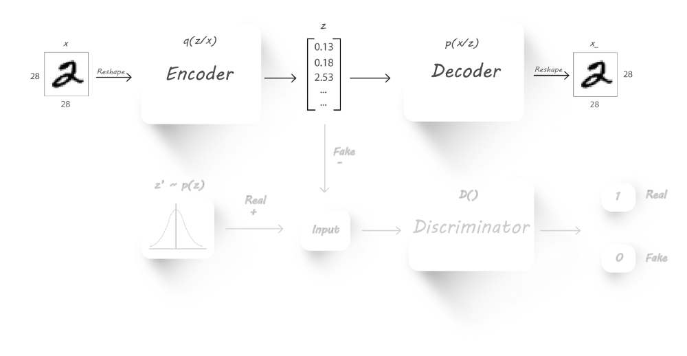
在该阶段，我们需要训练encoder和decoder来最小化重构误差（输入图片与重构图片间的均方误差）。我们将输入传递给encoder，encoder输出一个潜在码；随后，我们将该潜在码送入decoder从而得到一张重构图像。

正则化阶段

1__pIXKcCCqJRNmIWTRymJzA

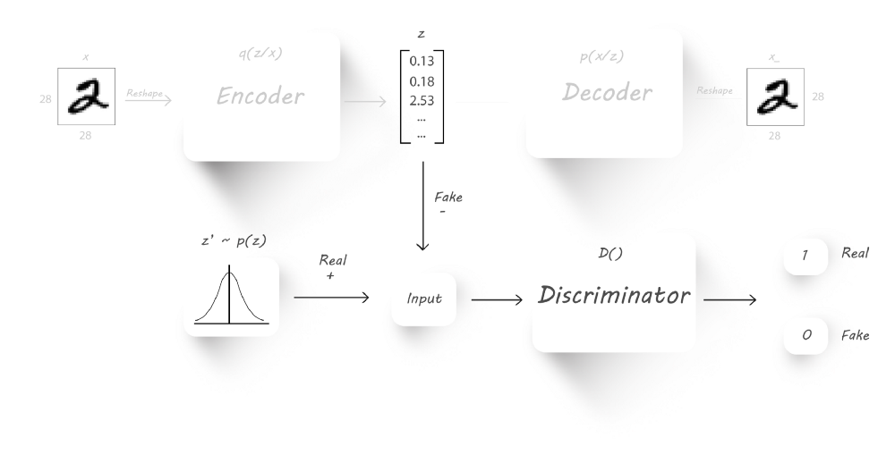
在该阶段，我们训练生成器和辨别器，我们将encod的输出$z$和随机采样$z’$（来自于想要的分布）作为输入来训练辨别器，这样辨别器就会返回1如果输入是$z’$，而返回0如果输入是$z$。接下来，为了迫使encoder的输出$z$逼近我们想要的分布，我们将encoder的输出作为辨别器的输入，连接encoder和辨别器。

1_DoJESN2LvxpxNVYADRJXWw

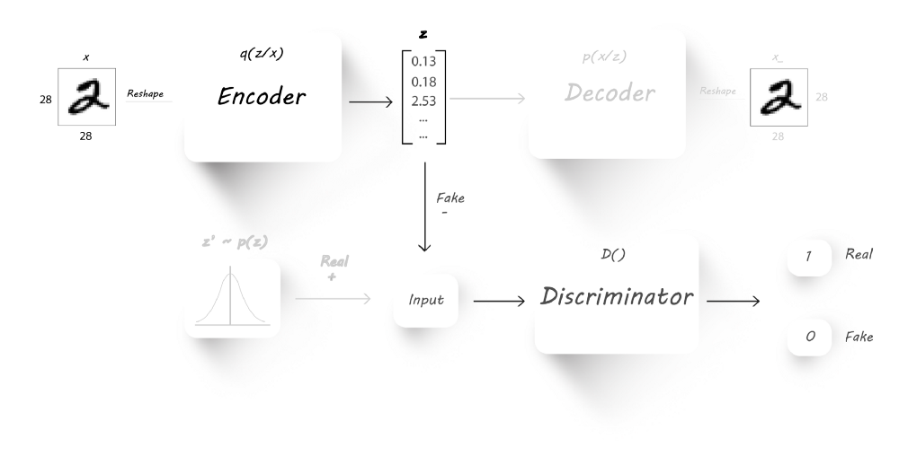
我们固定辨别器的权重参数，固定输入的目标标签为1，然后我们输入一些图像到encoder，并计算辨别器的输出与目标标签间的差异（使用交叉熵损失函数），这个阶段我们只更新encoder的权重参数，这样促使encoder去学习我们想要的分布，使输出服从这个分布。

Python实现

Encoder构造

1_Hud7t2vLY2JIP3SXn4WTDA

点击显/隐内容

def make_encoder(self):
    input_img = Input(self.input)
    h = Flatten()(input_img)
    h = Dense(1000,activation='relu')(h)
    h = Dense(1000,activation='relu')(h)
    mean = Dense(2)(h)
    logvar = Dense(2)(h)
    z = Lambda(self.sampling, output_shape=(self.latent_dim,))([mean, logvar])
    encoder = Model(input_img,z)
    encoder.summary()
    return encoder

def sampling(self, args):
    z_mean, z_log_sigma = args
    epsilon = K.random_normal(shape=(K.shape(z_mean)[0], self.latent_dim), mean=0., stddev=1.0)
    return z_mean + K.exp(z_log_sigma / 2) * epsilon

Decoder构造

1_0t7JrvUqyzg7AdQGDjZkRw

点击显/隐内容

def make_decoder(self): # ok
    input_code = Input((self.latent_dim,))
    h = Dense(1000,activation='relu')(input_code)
    h = Dense(1000,activation='relu')(h)
    h = Dense(784,activation='sigmoid')(h)
    recon_img = Reshape(self.input)(h)
    decoder = Model(input_code,recon_img)
    decoder.summary()
    return decoder

Discriminator构造

1_Df3_l66beZqsqRe5i6lZRw

点击显/隐内容

def make_discriminator(self): # ok
    input_code = Input((self.latent_dim,))
    h = Dense(1000,activation='relu')(input_code)
    h = Dense(1000,activation='relu')(h)
    valid = Dense(1)(h)
    discriminator = Model(input_code,valid)
    discriminator.summary()
    return discriminator

GAN的构造与编译

点击显/隐内容

class aae():
    def __init__(self):
        self.input = (28,28,1)
        self.latent_dim = 2
        optimizer = Adam(lr=0.0002,beta_1=0.5)

        # Build and compile the discriminator
        self.discriminator = self.make_discriminator()
        self.discriminator.compile(optimizer=optimizer,
                                   loss=['binary_crossentropy'],
                                   metrics=['accuracy'])

        # Build the encoder / decoder
        self.encoder = self.make_encoder()
        self.decoder = self.make_decoder()
        image = Input(self.input)
        latent_code = self.encoder(image)
        recon_img = self.decoder(latent_code)

        # for the adversarial_autoencoder model, we only train the generator
        self.discriminator.trainable = False
        valid = self.discriminator(latent_code)

        # The adversarial_autoencoder model  (stacked generator and discriminator)

        self.adversarial_autoencoder = Model(image,[recon_img,valid])
        self.adversarial_autoencoder.compile(loss=['mae','binary_crossentropy'],
                                             loss_weights=[0.999,0.001],
                                             optimizer=optimizer)

def train(self,epoches=1000,batch_size=100):

    # Load the dataset
    (X_train, _), (_, _) = mnist.load_data()
    # Configure input
    X_train = (X_train.astype(np.float32) - 127.5) / 127.5 # pixel between [-1,1]
    X_train = np.expand_dims(X_train, axis=3) # change shape from (60000,28,28) to (60000,28,28,1)
    # Adversarial ground truths
    valid = np.ones((batch_size, 1))
    fake = np.zeros((batch_size, 1))
    for epoch in range(1,epoches+1):
        # Select a random half batch of images
        idx = np.random.randint(0, X_train.shape[0], batch_size)
        imgs = X_train[idx]

        latent_fake = self.encoder.predict(imgs)
        latent_real = np.random.normal(0, 1, (batch_size, 2))

        # train the discriminator
        d_loss_real = self.discriminator.train_on_batch(latent_real, valid)
        d_loss_fake = self.discriminator.train_on_batch(latent_fake, fake)
        d_loss = 0.5 * np.add(d_loss_real, d_loss_fake)

        # train the generator
        g_loss = self.adversarial_autoencoder.train_on_batch(imgs, [imgs, valid])
        print("%d [D loss: %f, acc: %.2f%%] [G loss: %f, mse: %f]" % (
        epoch, d_loss[0], 100 * d_loss[1], g_loss[0], g_loss[1]))

1
2
3

if __name__ == '__main__':
    model = aae()
    model.train()

监督AAE

Disentanglement of style and content

对于一个写作主题，每一个人写出来的文章都有不同的内容（content）和字体（style）。对于MNIST字体，可以发现它的所有图像都有一样的style，所以我们想要从这个数据集中学习MNIST字体的style。为了更明确content和style的区别，我们有如下图：

Screen Shot 2018-08-28 at 11.39.06 AM

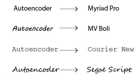
每个文本都有相同的content “Autoencoder”，但是它们的字体是不一样的，现在我们想要从图片中去区分style（Myriad Pro, MV Boil,…）和content，特征分离是表征学习(representation learning)的一个重要内容。

Autoencoder和Adversarial Autoencoder都是无监督学习，因为在训练过程中我们并没有世人任何label信息，但是如果利用图片的label信息则会帮助AAE去提取style信息而不受图片content的影响，这样我们的AAE就变成了一个监督模型。

模型

1_vGU0REkvre1DI7sFLU97_g

除了利用latent code作为decoder的输入，我们同时把标签y信息作为另一个输入，decoder利用这两个输入来生成图片。encoder学习图片的style，decoder利用该学习到的style和额外的内容信息y来重构输入图片

相比较于无监督AAE，唯一的区别就是decoder的输入：

来自encoder的latent code
图像标签的独热表示

训练

重构阶段

我们将输入图像送入encoder得到输出latent codez，然后将z和图像标签y串接起来成为一个更大的输入送入decoder。我们训练AE使最小化图片重构损失

正则化阶段

与无监督 AAE一样。

Python实现

Decoder

1_lzIl05QPdy-aEtVvh-y1LQ

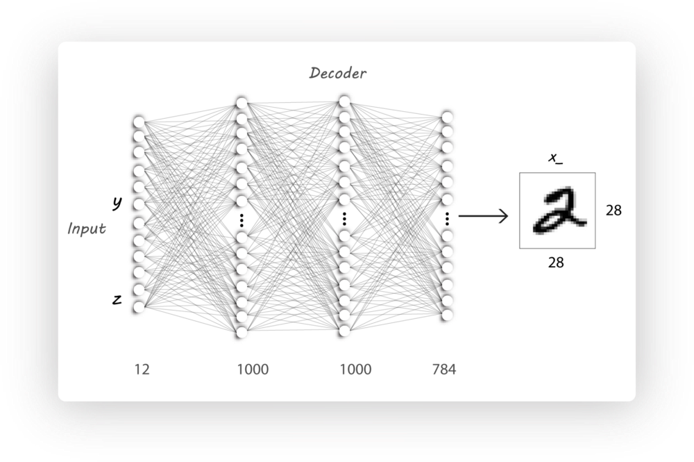
MNIST的图像总共有10类，则y的独热向量长度就是10，laten code的长度是2，则decoder的输入长度是（10+2）

点击显/隐内容

from keras.datasets import mnist
from keras.layers import Input, Dense, Reshape, Flatten, Dropout, multiply
from keras.layers import BatchNormalization, Embedding, Lambda,Concatenate
from keras.layers.advanced_activations import LeakyReLU
from keras.models import Sequential, Model
from keras.optimizers import Adam
from keras import backend as K
import keras
import matplotlib.pyplot as plt
import os
import numpy as np

class aae():
    def __init__(self):
        self.input = (28,28,1)
        self.latent_dim = 15
        self.classes = 10
        optimizer = Adam(lr=0.0002,beta_1=0.5)

        # Build and compile the discriminator
        self.discriminator = self.make_discriminator()
        self.discriminator.compile(optimizer=optimizer,
                                   loss=['binary_crossentropy'],
                                   metrics=['accuracy'])

        # Build the encoder / decoder
        self.encoder = self.make_encoder()
        self.decoder = self.make_decoder()
        image = Input(self.input)
        label = Input((self.classes,))
        latent_code = self.encoder(image)
        recon_img = self.decoder([label,latent_code])

        # for the adversarial_autoencoder model, we only train the generator
        self.discriminator.trainable = False
        valid = self.discriminator(latent_code)

        # The adversarial_autoencoder model  (stacked generator and discriminator)

        self.adversarial_autoencoder = Model([image,label],[recon_img,valid])
        self.adversarial_autoencoder.compile(loss=['mse','binary_crossentropy'],
                                             loss_weights=[0.999,0.001],
                                             optimizer=optimizer)

    def sampling(self, args):
        z_mean, z_log_sigma = args
        epsilon = K.random_normal(shape=(K.shape(z_mean)[0], self.latent_dim), mean=0., stddev=1.0)
        return z_mean + K.exp(z_log_sigma / 2) * epsilon

    def make_encoder(self):
        input_img = Input(self.input)
        h = Flatten()(input_img)
        h = Dense(1000,activation='relu')(h)
        h = Dense(1000,activation='relu')(h)
        mean = Dense(self.latent_dim)(h)
        logvar = Dense(self.latent_dim)(h)
        z = Lambda(self.sampling, output_shape=(self.latent_dim,))([mean, logvar])
        encoder = Model(input_img,z)
        encoder.summary()
        return encoder
    def make_decoder(self): # ok
        input_code = Input((self.latent_dim,))
        input_label = Input((self.classes,))
        combine_input = Concatenate(axis=-1)([input_label, input_code])
        h = Dense(1000,activation='relu')(combine_input)
        h = Dense(1000,activation='relu')(h)
        h = Dense(784,activation='sigmoid')(h)
        recon_img = Reshape(self.input)(h)
        decoder = Model([input_label,input_code],recon_img)
        decoder.summary()
        return decoder
    def make_discriminator(self): # ok
        input_code = Input((self.latent_dim,))
        h = Dense(1000,activation='relu')(input_code)
        h = Dense(1000,activation='relu')(h)
        valid = Dense(1)(h)
        discriminator = Model(input_code,valid)
        discriminator.summary()
        return discriminator
    def train(self,epoches=1000,batch_size=100):

        # Load the dataset
        (X_train, y_train), (_, _) = mnist.load_data()
        # Configure input
        X_train = (X_train.astype(np.float32) - 127.5) / 127.5 # pixel between [-1,1]
        X_train = np.expand_dims(X_train, axis=3) # change shape from (60000,28,28) to (60000,28,28,1)
        y_train = y_train.reshape(-1, 1)
        # Adversarial ground truths
        valid = np.ones((batch_size, 1))
        fake = np.zeros((batch_size, 1))
        for epoch in range(1,epoches+1):
            # Select a random half batch of images
            idx = np.random.randint(0, X_train.shape[0], batch_size)
            imgs = X_train[idx]
            labels = y_train[idx]
            labels = keras.utils.to_categorical(labels,self.classes)

            latent_fake = self.encoder.predict(imgs)
            latent_real = np.random.normal(0, 5., (batch_size, self.latent_dim))

            # train the discriminator
            d_loss_real = self.discriminator.train_on_batch(latent_real, valid)
            d_loss_fake = self.discriminator.train_on_batch(latent_fake, fake)
            d_loss = 0.5 * np.add(d_loss_real, d_loss_fake)

            # train the generator
            g_loss = self.adversarial_autoencoder.train_on_batch([imgs,labels], [imgs, valid])
            print("%d [D loss: %f, acc: %.2f%%] [G loss: %f, mse: %f]" % (
            epoch, d_loss[0], 100 * d_loss[1], g_loss[0], g_loss[1]))

if __name__ == '__main__':
    model = aae()
    model.train()

GAN分类器

ref

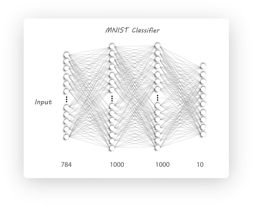
本节我们将介绍如何利用encoder对MNIST手写体进行分类，并与传统的神经网络分类器(NN)比较，为保证实验公平性，encoder和NN使用相同的结构。

我们首先介绍传统的NN分类器，如下图所示，

1_OPtU8py5KBpbVUZKylGDPA

点击显/隐内容

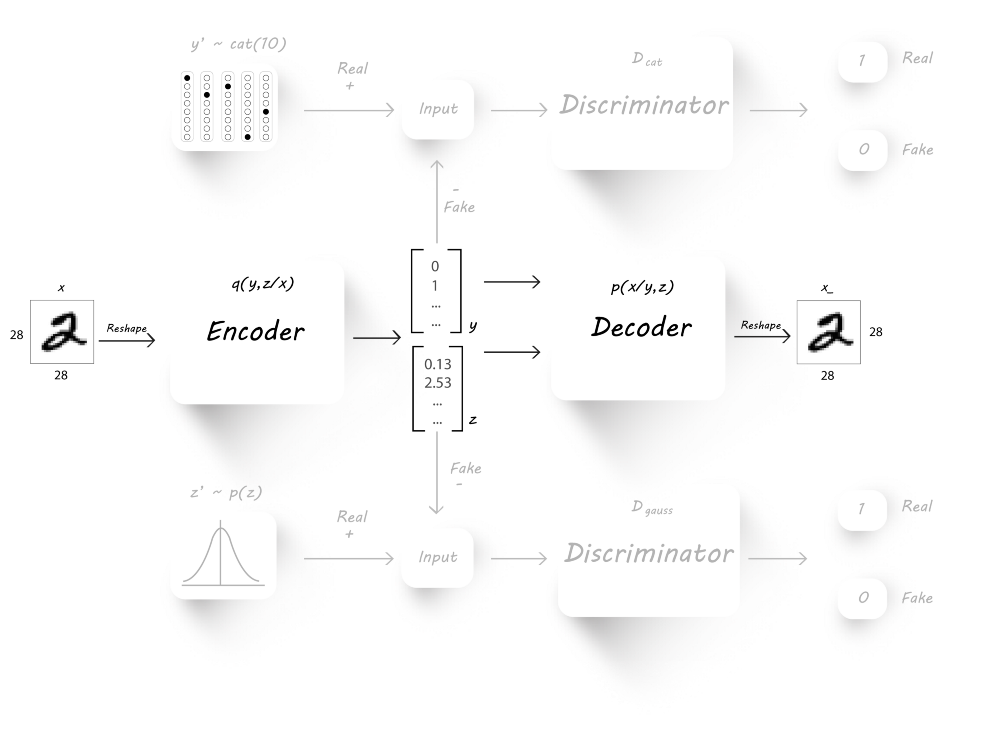
那么我们如何将encoder改造成为一个分类器呢？实际上，encoder分类器不仅能够提升分类准确率，还可以减少数据维度，从图片中分离内容和风格，我们的模型如下：

1_8RuZ8kguLuosOGoDpiSgUQ

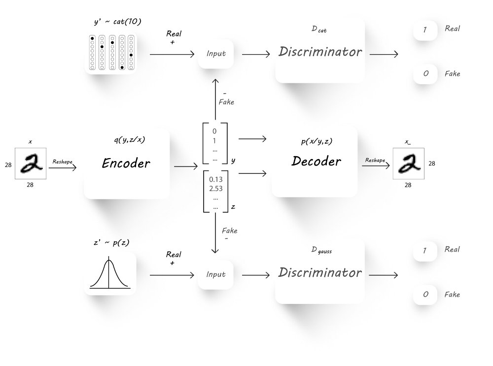
可以看到，我们增加了额外的discriminator（$D_{cat}$），该分类器以对抗的方式与encoder一起训练，从而迫使encoder产生10维的独热分类向量

在AAE的基础上对encoder作了修改，此时encoder有两个输出：latent code（z）和classification（y），由于有10个类，则y为10维向量，而z的维度由用户决定。

图片重构阶段

1_onLoFTa8qcFMdgm9ILKDaw

该阶段我们欲使生成的图片逼近我们的真实图片，所以我们使用MSE（mean squared error）来衡量输入图片与输出图片间的差异。

正则化阶段

该阶段由两个部分组成：$D_{cat}$和$D_{gauss}$的训练

1_HKvMbwaXmDAg12GjgOC39Q

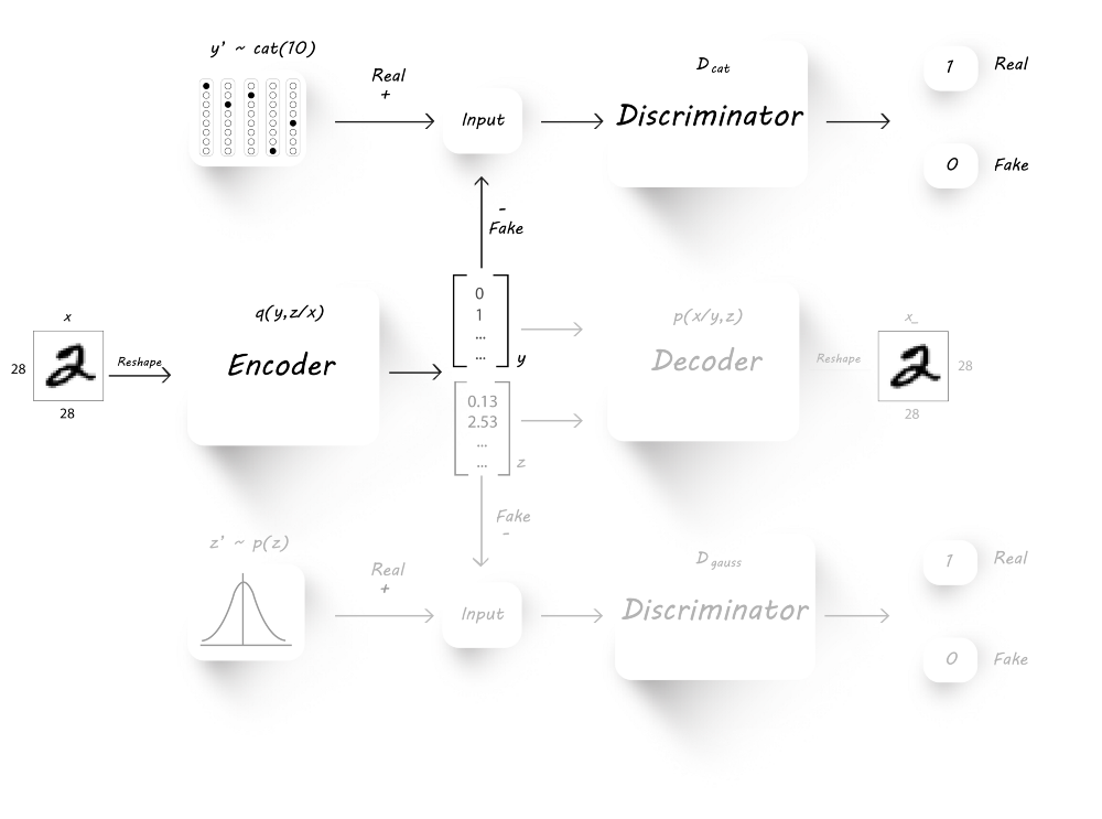
我们首先训练discriminator D_cat来辨别真实的分类标签$y^{‘}$和encoder生成的分类标签$y$。为此，我们将图片作为encoder的输入取产生$y$和$z$，然后将生成的$y$和真实的$y^{‘}$用于discriminator的训练。最后，我们固定分辨器的参数，并设置目标为1，训练encoder来欺骗分辨器。

1_qMGBvI2q14lNKGMrx_gMnw

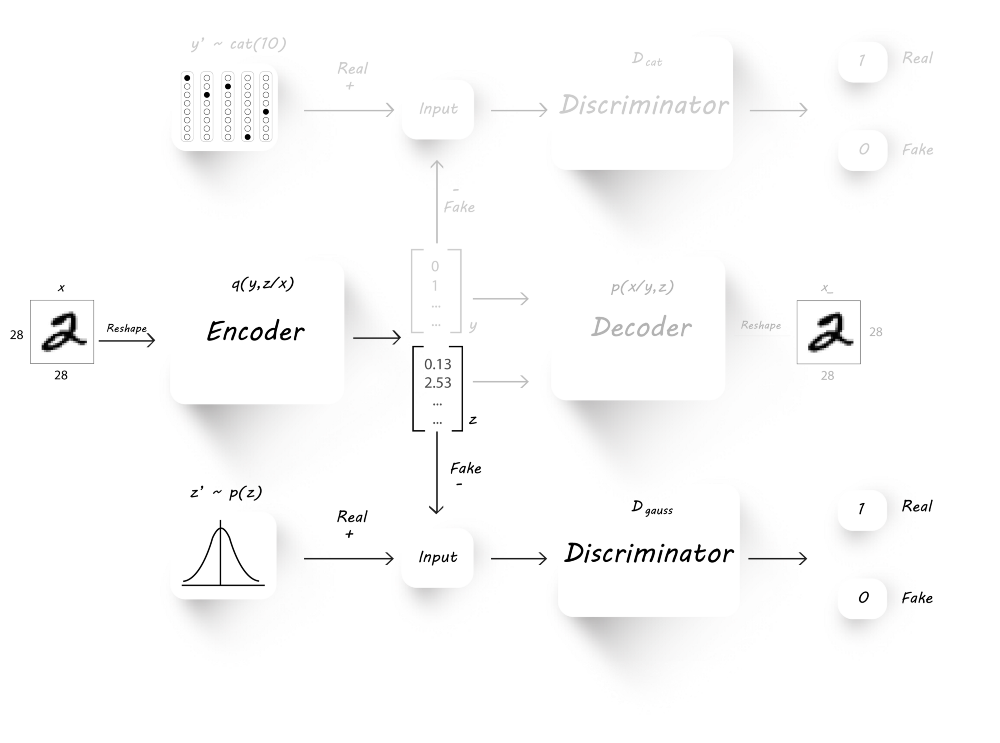
同样的，为了生成具有高斯分布的latent code（z），我们还需要训练分辨器$D_{gauss}$。

半监督分类器阶段

1_ZS7wa7H8tHUDWkuqGZJT2Q

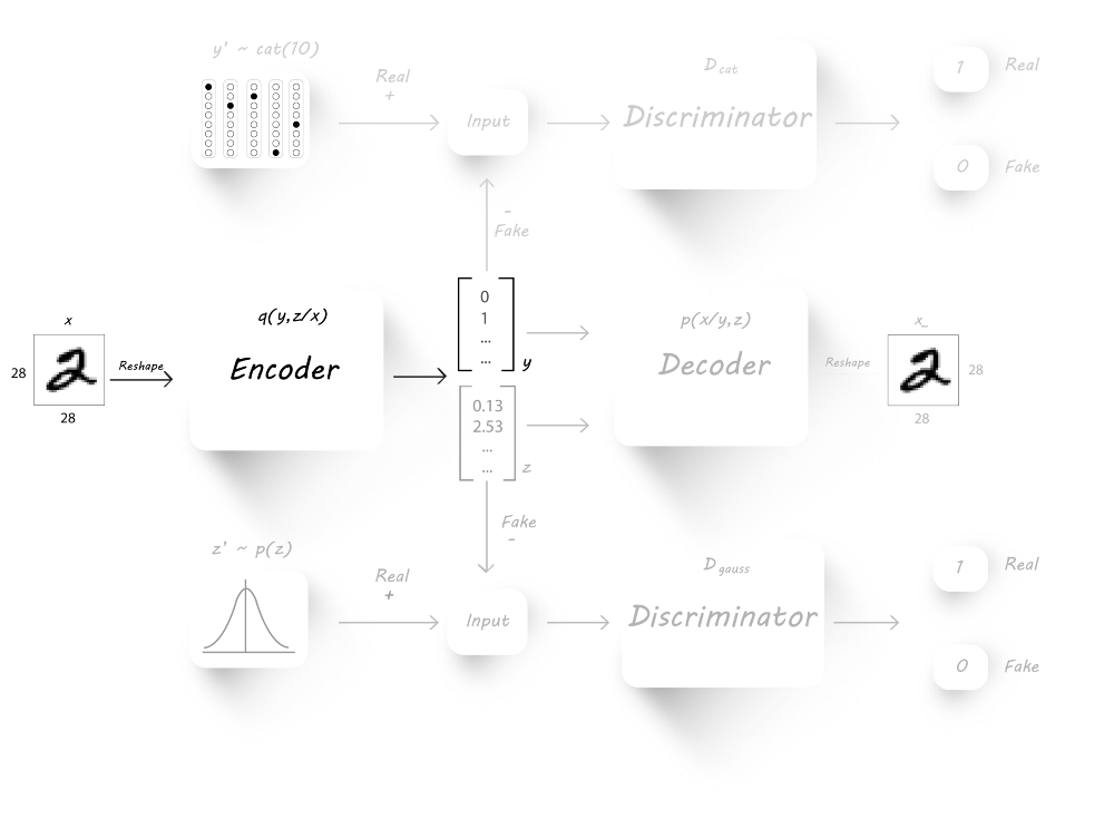
最终我们训练encoder来对手写体数字进行分类，目的是最小化生成的分类标签与真实的标签的交叉熵。

Python实现

Encoder

1_qufKKgKUPUGvYKWsmqiv5w

在原始encoder的基础上，只需要需改encoder的输出维度，增加对分类标签的输出

Decoder

1_nRF013A75pCdlgOT48w0MA

Discriminator

1_jzDB_IJhVL74Zb0NU03Uew

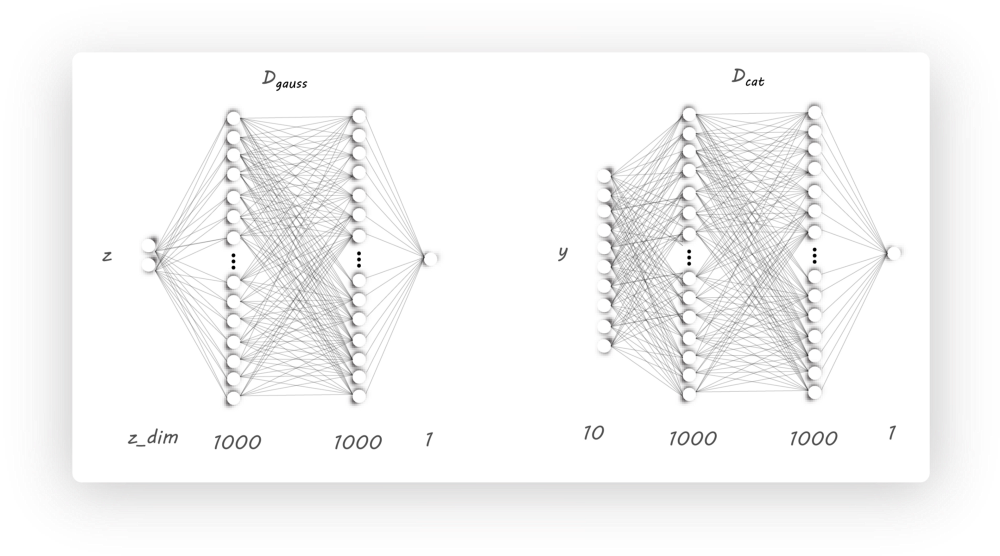
我们需要两个分辨器，它们除了输入维度不同，其他是一样的

点击显/隐内容

CVAE-GAN

REF1

《 CVAE-GAN: Fine-Grained Image Generation through Asymmetric Training》

点击显/隐内容

Linear Regression

Posted on 2018-08-06 | In Machine Learning

线性回归

模型

线性回归模型，顾名思义就是线性模型求解回归问题。

线性模型

【定义】给定具有$d$个属性的数据样本$x=\{x_1,x_2,…,x_d\}$，$x_i$是$x$在第$i$个属性上的取值，线性模型通过对属性的线性组合来进行预测的函数：

$f(x)=w_1x_1+w_2x_2+...+w_dx_d+b$

向量形式表示为：

$f(x)=w^Tx+b$

其中$w=(w_1;w_2;…;w_d)$，只要确定了$w$和$b$，模型就得以确定。

向量都表示成竖直的一条直线。

回归问题

回归属于监督学习的范畴，用于预测输入变量与输出变量的关系。其本质就是数据拟合，选择一条函数曲线使其很好地拟合已知的数据，同时能够预测未知的数据。

按照输入变量的属性个数，分为一元回归和多元回归；按照输入变量和输出变量之间的映射关系，分为线性回归和非线性回归。

线性回归

线性模型描述的是属性间的组合关系，而回归问题求解的是输入与输出的关系。

即使用一个线性函数去建模输入变量属性间的线性关系，从而发现输入变量与输出变量的关系。给定数据集$D=\{(x_1,y_1),(x_2,y_2),…,(x_m,y_m)\}$，其中$x_i=(x_i1;x_i2;…;x_id)$。

问题描述：线性回归试图学习一个线性模型$f(x_i)=w^Tx_i+b$，使$f(x_i)\approx y_i$。

又称为多元线性回归，或者多变量线性回归。

算法求解

最小二乘法

只要确定了权重$w$和偏差$b$的值，那么我们就可以得到模型了，而我们想让预测值$f(x_i)$无限接近真实值$y_i$，所以使用均方误差作为性能度量，即我们试图让均方差最小：

$Loss(w^*,b^*)=\sum_{i=1}^{m}(f(x_i)-y_i)^2$

均方误差对应了常用的欧几里得距离，基于均方误差最小化进行模型求解的方法称为“最小二乘法”，实际上，最小二乘法就是试图找到一条直线，使样本到直线的欧氏距离之和最小。

关于为什么使用均方误差作为损失度量，一个是因为其本质是最大似然法，ref

常用损失函数对比ref2

参数估计

Loss函数求导取极值

我们可以对损失函数$Loss$求导，并令导数为零来求得最优参数：

$\begin{cases} w=\frac{\sum_{i=1}^{n}y_i(x_i-\bar{x})}{\sum_{i=1}^{n}x_{i}^{2}-\frac{1}{n}(\sum_{i=1}^{n}x_i)^2}\\ b=\frac{1}{m}\sum_{i=1}^{n}(y_i-wx_i) \end{cases}$

点击显/隐内容

公式推导

偏导
$\begin{cases} \frac{\partial{}E}{\partial{w}}=2[w\sum_{i=1}^{n}x_{i}^{2}-\sum_{i=1}^{n}(y_i-b)x_i]\\ \frac{\partial{}E}{\partial{b}}=2[mb-\sum^{n}_{i=1}(y_i-wx_i)] \end{cases}$
求解b，$\frac{\partial{}E}{\partial{b}}=0$
$\begin{align*} mb&=\sum^{n}_{i=1}(y_i-wx_i)\\ &=(y_1-wx_1)+(y_2-wx_2)+...+(y_n-wx_n)=(y_1+y_2+...+y_n)-w(x_1+x_2+...+x_n)\\ &=\sum{y_i}-w\sum{x_i} \end{align*}$
则$b=\frac{1}{n}\sum_{i=1}^{n}(y_i-wx_i)=\bar{y}-w\bar{x}$
求解w，$\frac{\partial{}E}{\partial{w}}=0$
$\begin{align*} w\sum_{i=1}^{n}x_{i}^{2}&=\sum_{i=1}^{n}(y_i-\bar{y}+w\bar{x})x_i\\ &=(y_1-\bar{y}+w\bar{x})x_1+(y_2-\bar{y}+w\bar{x})x_2+...+(x_n-\bar{y}+w\bar{x})x_n\\ &=(y_1x_1+y_2x_2+...+y_nx_n)-\bar{y}(x_1+x_2+...+x_n)+w\bar{x}(x_1+x_2+...+x_n)\\ &=\sum_{i=1}^{n}x_iy_i-\bar{y}\sum_{i=1}^{n}x_i+w\bar{x}\sum_{i=1}^{n}x_i\\ &=\sum_{i=1}^{n}x_iy_i-n\bar{y}\bar{x}+w\bar{x}n\bar{x} \end{align*}$
则$w(\sum_{i=1}^{n}x_{i}^{2}-n\bar{x}^2)=\sum_{i=1}^{n}x_iy_i-n\bar{y}\bar{x}$，故
$w=\frac{\sum_{i=1}^{n}x_iy_i-n\bar{y}\bar{x}}{\sum_{i=1}^{n}x_{i}^{2}-n\bar{x}^2}$

梯度下降法

损失函数是：

$\begin{align*} Loss(w,b)&=\sum_{i=1}^{n}(f(x_i)-y_i)^2\\ &=\sum_{i=1}^{n}(wx_i+b-y_i)^2 \end{align*}$

参数更新：

$\begin{cases} w=w-\alpha(f(x)-y){x}\\ b=b-\alpha(f(x)-y) \end{cases}$

$\begin{align*} \frac{\partial{E}}{\partial{w}}&=\frac{\partial{}}{\partial{w}}{\frac{1}{2}(f(x)-y)^2}\\ &=(f(x)-y)\frac{\partial}{\partial{w}}(wx+b-y)\\ &=(f(x)-y)x \end{align*}$

即：

$w_i=w_i-\alpha\frac{1}{m}\sum_{i=1}^{m}(f(x_i)-y_i)\cdot x_i$

此时，$b=w_0$，$x_0=1$。

正则化的损失函数

此时目标函数为：

$\begin{align*} E(w,b)&=\sum_{i=1}^{n}(wx_i+b-y_i)^2+\lambda\sum_{i=1}^{n}w_{i}^{2} \end{align*}$

$w_0$不需要正则化

此时梯度下降法为：

$w_0=w_0-\alpha\frac{1}{n}\sum_{i=1}^{n}(h_w(x^{(i)})-y^{(i)})x_0^{(i)}\\ w_j=w_j-\alpha[\frac{1}{n}\sum_{i=1}^{n}(h_w(x^{(i)})-y^{(i)})x_j^{(i)}-\frac{\lambda}{n}w_j]$

Data Preprocessing

Feature Scaling

It involves dividing the input values by the range (i.e. the maximum value minus the minimum value) of the input variable, resulting in a new range of just 1.

Mean normalization

This involves subtracting the average value for an input variable from the values for that input variable resulting in a new average value for the input variable of just zero.

By combining the two techniques and adjust the input values as shown in the following formula:

$x_i=\frac{x_i-\mu_i}{s_i}$

where $\mu_i$ is the average of all the values for feature $(i)$ and $s_i$ is the range of values (max - min), or $s_i$ is the standard deviation.

Convergence Figure

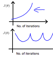
In order to make sure that our algorithm runs correctly, we need to debug gradient descent. Make a plot with number of iterations on the x-axis. Now plot the cost function, $J(\theta)$ over the number of iterations of gradient descent. If $J(\theta)$ ever increases, then you probably need to decrease learning rate $\alpha$.

Summary

If $\alpha$ is too small, it could result in slow convergence.
If $\alpha$ is too large, it may not decrease on every iteration and thus may not converge, like the following pic:

Screen Shot 2018-08-06 at 12.58.12 PM

Example

Screen Shot 2018-08-06 at 12.54.04 PM

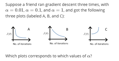
A is $\alpha=0.1$, B is $\alpha=0.01$, A is $\alpha=1$.

In graph C, the cost function is increasing, so the learning rate is set too high. Both graphs A and B converge to an optimum of the cost function, but graph B does so very slowly, so its learning rate is set too low. Graph A lies between the two.

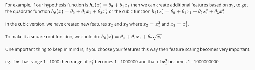
Polynomial Regression

Our hypothesis function need not be linear (a straight line) if that does not fit the data well.

We can change the behavior or curve of our hypothesis function by making it a quadratic, cubic or square root function (or any other form).

Screen Shot 2018-08-07 at 12.18.01 AM

例子

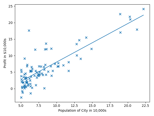
线性回归预测一维数据

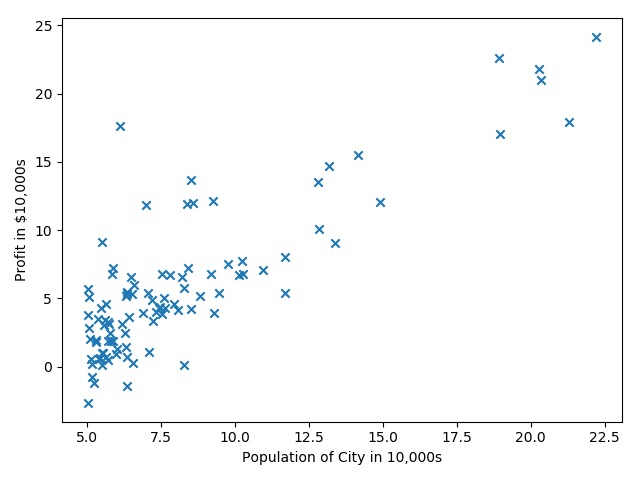
来自Andrew Ng第二周的课程练习，给出城市人口及该市的商店利润，预测如何进行店铺扩展，即选择哪座城市开分店？给定的数据只有一个人口特征及利润目标值。

第一步就是进行数据的可视化。

点击显/隐内容

def plot_data():
    data = np.loadtxt('./dataset/ex1data1.txt', delimiter=',')
    x = data[:, 0]
    y = data[:, 1]
    plt.scatter(x, y, marker='x')
    plt.xlabel("Population of City in 10,000s")
    plt.ylabel("Profit in $10,000s")
    plt.show()

第二步：数据处理及参数初始化

我们为数据增加一列全一

点击显/隐内容

length = x.shape[0]
z = np.ones(length)
x = np.array(list(zip(z,x)))  # add a column of ones to x
theta = np.zeros([x.shape[1],1]) # initialize fitting parameters
alpha = 0.01
iters = 1500

第三步：损失函数

我们使用公式

Screen Shot 2018-08-15 at 6.19.39 PM

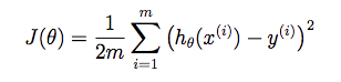
初次调用，返回值是32.07。

点击显/隐内容

def cost_function(x,y,theta):
    y_ = x.dot(theta)
    loss = (y-y_)**2
    cost = sum(loss) / (2*length)
    return cost

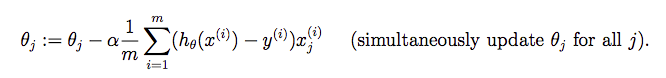
第四步：梯度下降法

检查梯度下降法是否正确的一个手段：查看损失函数是否在逐步减小。我们使用梯度更新公式：

Screen Shot 2018-08-15 at 6.26.20 PM

点击显/隐内容

def gradient_descent(x,y,theta,alpha,iters):
    for i in range(iters):
        # cost_function(x,y,theta)
        y_ = x.dot(theta)
        loss = (y_ - y)
        gd = loss.T.dot(x) # shape = (1,2)
        gd = alpha * gd.T / length
        theta = theta - gd
    return theta

需要注意的一个点是：loss = ( y_pred - y )。反过来的话，会出现loss趋于无穷大。这个是对loss函数求导得到的，无论$(h_\theta(x)-y )^2$还是$(y-h_\theta(x) )^2$，都是一样的。

第五步：可视化拟合曲线

点击显/隐内容

def plot_data(x,y,theta):
    plt.scatter(x, y, marker='x',label='Training data')
    plt.xlabel("Population of City in 10,000s")
    plt.ylabel("Profit in $10,000s")
    x_ = np.linspace(min(x),max(x),1000)
    y_ = x_*theta[1] + theta[0]
    plt.plot(x_,y_,label='Linear regression')
    plt.show()

线性回归预测多特征数据

我们使用线性回归预测房价，数据集有两个特征：第一列是房屋面积(单位：$feet^2$)，第二列是房间数，最后一列是房价。

特征正则化

发现两个特征数据范围相差特别大，所以需要对数据进行正则化，这样可以加快梯度下降法的收敛。

减去均值
除以标准差

正则化之后，别忘记加一个全一列。

注意：记得存储mean和std的值，这样我们在预测位置数据的时候，第一步就是使用mean和std对未知数据做同样的处理。

点击显/隐内容

def feature_norm(x):
    mean = np.mean(x,axis=0)
    std = np.std(x,axis=0)
    x = (x-mean)/std
    ones = np.ones((x.shape[0], 1))
    x = np.concatenate([ones, x], axis=1)
    return x,mean,std

梯度下降法

先实现损失函数

Screen Shot 2018-08-15 at 6.19.39 PM

点击显/隐内容

def cost_func(x,y,thetas):
    y_pred = x.dot(thetas)
    loss = sum((y_pred-y)**2)/(2*x.shape[0])
    return loss

再实现梯度下降法，损失函数都是10次方。

点击显/隐内容

def gradient_dec(x,y,thetas,lr,iter):
    for i in range(iter):
        y_pred = x.dot(thetas)
        gd = (y_pred - y).T.dot(x)
        thetas -= lr * gd.T / x.shape[0]
        loss = cost_func(x, y, thetas)
        print(loss)
    return thetas

Linux命令

Posted on 2018-08-05 | In Linux

文件

退出保存

:wq

利用scp远程上传下载文件/文件夹ref1

统计文件个数

1 2	ls -l \|grep "^-"\|wc -l #统计当前目录下文件数量 ls -l \|grep "^ｄ"\|wc -l #统计当前目录下文件夹数量

1	cp -r dir1/. /dir2/

设置屏幕分辨率

1	xrandr -s 1366x768

删除

删除目录下所有文件

用通配符*英文星号可以表示“所有文件”这个概念，所以删除文件夹下所有文件的方法就是，先用cd命令切换到这个文件夹下，然后执行rm ./*命令表示删除当前目录下所有的文件，但是注意，如果文件夹下有子目录，这条命令就无法生效了，因为它无法删除子目录（删除子目录要加上-r选项）。

Training Techiniques

Posted on 2018-08-03 | In Deep Learning

Techniques for training a Deep Learning model.

Keras

Posted on 2018-07-23 | In Deep Learning

Keras使用技巧。

TODO

[ ] LSTM
[ ] CONV1D
[ ] TIMEDISTRIBUTED-VIDEOS
[ ] FIT_GENERATOR
[ ] STATEFUL_RNN

AutoEncoder

Posted on 2018-07-22 | In Deep Learning

AutoEncoder通过设计encode和decode过程使输入和输出越来越接近，是一种自监督学习过程，输入图片通过encode进行处理，得到code，再经过decode处理得到输出，我们可以控制encode的输出维数，就相当于强迫encode过程以低维参数学习高维特征。

Generative Adversarial Networks

Posted on 2018-07-20 | In Deep Learning

Richard Feynman说“如果要真正理解一个东西，我们必须要能够把它创造出来。”

GAN 启发自博弈论中的二人零和博弈（two-player game），GAN 模型中的两位博弈方分别由生成式模型（generative model）和判别式模型（discriminative model）充当。生成模型 G 捕捉样本数据的分布，用服从某一分布（均匀分布，高斯分布等）的噪声 z 生成一个类似真实训练数据的样本，追求效果是越像真实样本越好；判别模型 D 是一个二分类器，估计一个样本来自于训练数据（而非生成数据）的概率，如果样本来自于真实的训练数据，D 输出大概率，否则，D 输出小概率。

Variational AutoEncoder

Posted on 2018-07-20 | In Deep Learning

AutoEncoder（自编码器）本质上是数据特定的数据压缩。虽然自编码器中的重构损失函数确保了编码过程原始数据不会丢失过多，但是没有对约束特征$z$做出约束。

作为一种无监督的学习方法，VAE（Variational Auto-Encoder，变分自编码器）是一个产生式模型，其在ae的基础上约束潜变量$z$服从于某个已知的先验分布$p(z|x)$，比如希望$z$的每个特征相互独立并且符合高斯分布等。

EasyDict

目录

R & W in TXT

文件操作

文件移动

Print

pprint

Random

np.random.rand()

np.random.randn()

np.random.randint()

np.random.choice()

String

数字补0

Plt

Time

Zip

Parser

Matplotlib

ElementTree

Naming style

Adversarial Autoencoder

无监督AAE

模型

训练

重构阶段

正则化阶段

Python实现

Encoder构造

Decoder构造

Discriminator构造

GAN的构造与编译

监督AAE

模型

训练

重构阶段

正则化阶段

Python实现

Decoder

GAN分类器

图片重构阶段

正则化阶段

半监督分类器阶段

Python实现

Encoder

Decoder

Discriminator

CVAE-GAN

线性回归

模型

线性模型

回归问题

线性回归

算法求解

最小二乘法

参数估计

Loss函数求导取极值

梯度下降法

正则化的损失函数

Data Preprocessing

Convergence Figure

Polynomial Regression

例子

线性回归预测一维数据

线性回归预测多特征数据

特征正则化

梯度下降法

文件

删除